
Project 4 · Unsupervised Learning
How Amazon Knows What Kind of Customer You Are
Turn raw retail transactions into customer groups without a pre-existing target label. You will build the RFM table, choose a defensible number of clusters, compare three clustering ideas, interpret the groups, and ship a working app.
The practical problem: thousands of shoppers, but no customer labels
Imagine an online retailer has more than half a million transaction rows. Marketing cannot treat every customer exactly the same, but nobody has supplied labels such as “VIP”, “occasional” or “at risk”. We therefore cannot train an ordinary classifier. Our job is to turn purchase history into measurable behaviour, discover natural groups, and explain what those groups actually mean.
Raw evidence
541,909 historical UCI retail transaction rows.
Behaviour features
Recency, Frequency and Monetary value for each known customer.
ML task
Unsupervised clustering: discover groups without a target column.
Deliverable
A saved K-Means segmenter plus a Streamlit app that assigns a new RFM profile.
What are we actually asking the algorithm to discover?
Recency (R)
How many days ago did this customer last buy? Smaller usually means more recently active.
Frequency (F)
How many distinct completed orders did this customer place? Larger means more repeat buying.
Monetary (M)
How much historical revenue came from this customer? Larger means greater historical spend.
Important: K-Means will return cluster IDs such as 0 and 1. It does not know words like “high-value”. We create business-friendly names only after examining the measured profile of each cluster.
Step 1: Create the project environment
Work inside projects/customer-segmentation. The versions below are the ones used by the verified build.
pandas==3.0.6
numpy==2.5.3
pyarrow==21.0.0
openpyxl==3.1.5
scikit-learn==1.9.1
matplotlib==3.11.2
joblib==1.6.0
streamlit==1.65.0
pytest==9.0.2
python -m venv .venv
.\.venv\Scripts\Activate.ps1
python -m pip install -r requirements.txt
python -m pip check
Check before continuing
Step 2: Download a real retail dataset reproducibly
We use UCI Online Retail, dataset 352. It contains transactions from a UK-based non-store retailer and is licensed CC BY 4.0. The downloader validates the exact schema and pins the downloaded archive fingerprint so a silent upstream data change cannot pass unnoticed.
"""Download and validate UCI Online Retail for the customer-segmentation project."""

from __future__ import annotations

from io import BytesIO
from pathlib import Path
import hashlib
import zipfile
import urllib.request

import pandas as pd

ROOT = Path(__file__).resolve().parent
DATA_DIR = ROOT / "data"
XLSX_PATH = DATA_DIR / "Online Retail.xlsx"
PARQUET_PATH = DATA_DIR / "online_retail.parquet"

SOURCE_URL = "https://archive.ics.uci.edu/static/public/352/online+retail.zip"
EXPECTED_ROWS = 541_909
EXPECTED_COLUMNS = [
    "InvoiceNo",
    "StockCode",
    "Description",
    "Quantity",
    "InvoiceDate",
    "UnitPrice",
    "CustomerID",
    "Country",
]
# Pin this after the first clean CI download. Until then the script prints the observed hash.
EXPECTED_ZIP_SHA256 = "f5385cbb54bbebf7196389109c6b0621faab0c304e3702548165e71c84aede8b"


def download_bytes(url: str) -> bytes:
    request = urllib.request.Request(
        url,
        headers={"User-Agent": "LearnMLAcademy-customer-segmentation-handbook/1.0"},
    )
    with urllib.request.urlopen(request, timeout=180) as response:
        return response.read()


def main() -> None:
    DATA_DIR.mkdir(parents=True, exist_ok=True)

    raw = download_bytes(SOURCE_URL)
    sha256 = hashlib.sha256(raw).hexdigest()
    if EXPECTED_ZIP_SHA256 and sha256 != EXPECTED_ZIP_SHA256:
        raise RuntimeError(
            "UCI dataset archive fingerprint changed: "
            f"{sha256}; expected {EXPECTED_ZIP_SHA256}. Review before continuing."
        )

    with zipfile.ZipFile(BytesIO(raw)) as archive:
        names = archive.namelist()
        workbook_name = next(
            (name for name in names if name.lower().endswith(".xlsx")),
            None,
        )
        if workbook_name is None:
            raise RuntimeError(f"Expected an XLSX workbook in archive, found: {names}")
        XLSX_PATH.write_bytes(archive.read(workbook_name))

    frame = pd.read_excel(XLSX_PATH, engine="openpyxl")
    if len(frame) != EXPECTED_ROWS:
        raise RuntimeError(
            f"Unexpected row count {len(frame):,}; expected {EXPECTED_ROWS:,}."
        )
    if list(frame.columns) != EXPECTED_COLUMNS:
        raise RuntimeError(
            f"Unexpected schema {list(frame.columns)!r}; expected {EXPECTED_COLUMNS!r}."
        )

    # Excel stores some identifier columns with mixed numeric/string values.
    # Normalize text identifiers before writing Parquet so Arrow does not
    # attempt to coerce cancellation invoice numbers such as "C536379" to int.
    for column in ["InvoiceNo", "StockCode", "Description", "Country"]:
        frame[column] = frame[column].astype("string")

    frame.to_parquet(PARQUET_PATH, index=False)

    print("UCI dataset: Online Retail (dataset 352)")
    print(f"Rows: {len(frame):,}")
    print(f"Columns: {len(frame.columns)}")
    print(f"CustomerID missing: {int(frame['CustomerID'].isna().sum()):,}")
    print(f"Archive SHA256: {sha256}")
    print(f"Saved workbook: {XLSX_PATH}")
    print(f"Saved parquet: {PARQUET_PATH}")


if __name__ == "__main__":
    main()
python download_data.pyRows: 541,909
CustomerID missing: 135,080
Archive SHA256: f5385cbb54bbebf7196389109c6b0621faab0c304e3702548165e71c84aede8bCheck before continuing
Step 3: Turn messy transactions into valid purchases
A transaction file is not yet a customer table. We remove rows without a customer ID, cancellation invoice numbers, non-positive quantities and non-positive prices. Then each line gets revenue = Quantity × UnitPrice.
def clean_transactions(frame):
    cleaned = frame.loc[
        frame["CustomerID"].notna()
        & ~frame["InvoiceNo"].str.upper().str.startswith("C")
        & (frame["Quantity"] > 0)
        & (frame["UnitPrice"] > 0)
    ].copy()

    cleaned["revenue"] = (
        cleaned["Quantity"].astype(float)
        * cleaned["UnitPrice"].astype(float)
    )
return cleanedCheck before continuing
Step 4: Build one behavioural row per customer
We take one day after the last transaction as the snapshot date. If a customer last bought on 1 December and the snapshot is 10 December, recency is 9 days. Frequency counts distinct completed invoices, while monetary value sums line-level revenue.
snapshot = cleaned["InvoiceDate"].max().normalize() + pd.Timedelta(days=1)

rfm = (
    cleaned.groupby("CustomerID", as_index=False)
    .agg(
        last_purchase=("InvoiceDate", "max"),
        frequency_orders=("InvoiceNo", "nunique"),
        monetary_value=("revenue", "sum"),
    )
)

rfm["recency_days"] = (
    snapshot - rfm["last_purchase"].dt.normalize()
).dt.daysCheck before continuing
Step 5: See why raw RFM values need preparation
Real RFM distributions
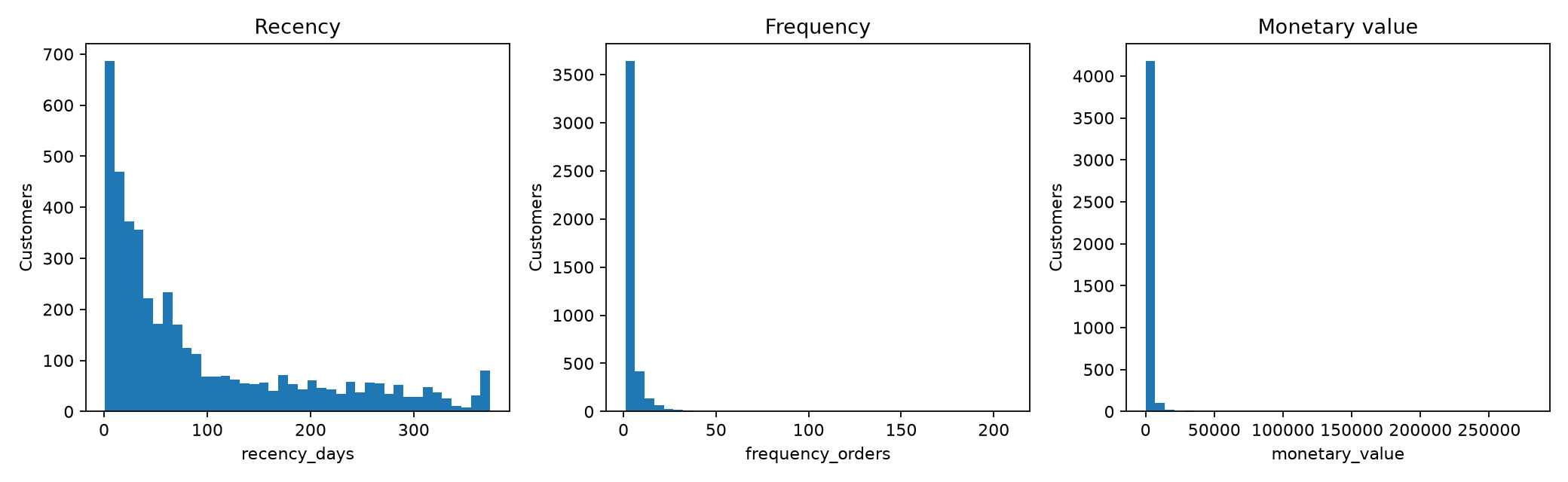
log1p before scaling.K-Means uses distances. If Monetary ranges into thousands while Frequency is mostly single digits, raw units can make spend dominate. A log transform compresses long right tails; StandardScaler then puts the three transformed features onto comparable standardized scales.
Check before continuing
Step 6: Log-transform and scale before distance-based clustering
logged = np.log1p(
    rfm[["recency_days", "frequency_orders", "monetary_value"]]
)

scaler = StandardScaler()
matrix = scaler.fit_transform(logged)
log1p(x) means log(1 + x), so it is safe at zero. StandardScaler then subtracts the training-column mean and divides by its standard deviation. We save that exact scaler with the final K-Means model so new profiles are transformed the same way.
Check before continuing
Step 7: Understand what K-Means is trying to minimize
Pick k cluster centres. Each customer is assigned to the nearest centre. The centre moves to the mean of its assigned customers. Assignment and movement repeat until the solution stabilizes. K-Means therefore favors compact groups in distance space; it does not discover business labels automatically.
Check before continuing
Step 8: Choose k with evidence instead of guessing
for k in range(2, 9):
    model = KMeans(
        n_clusters=k,
        n_init=20,
        random_state=42,
    )
    labels = model.fit_predict(matrix)

    score = silhouette_score(
        matrix,
        labels,
        sample_size=min(5000, len(matrix)),
        random_state=42,
    )
Real k-selection evidence
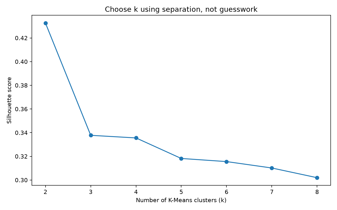
Silhouette compares how close a sample is to its own cluster versus neighboring clusters. Higher is generally better: values near +1 indicate better separation, values near 0 indicate overlap, and negative values suggest possible mis-assignment. It is a diagnostic, not proof that a business truly has exactly k natural customer types.
Check before continuing
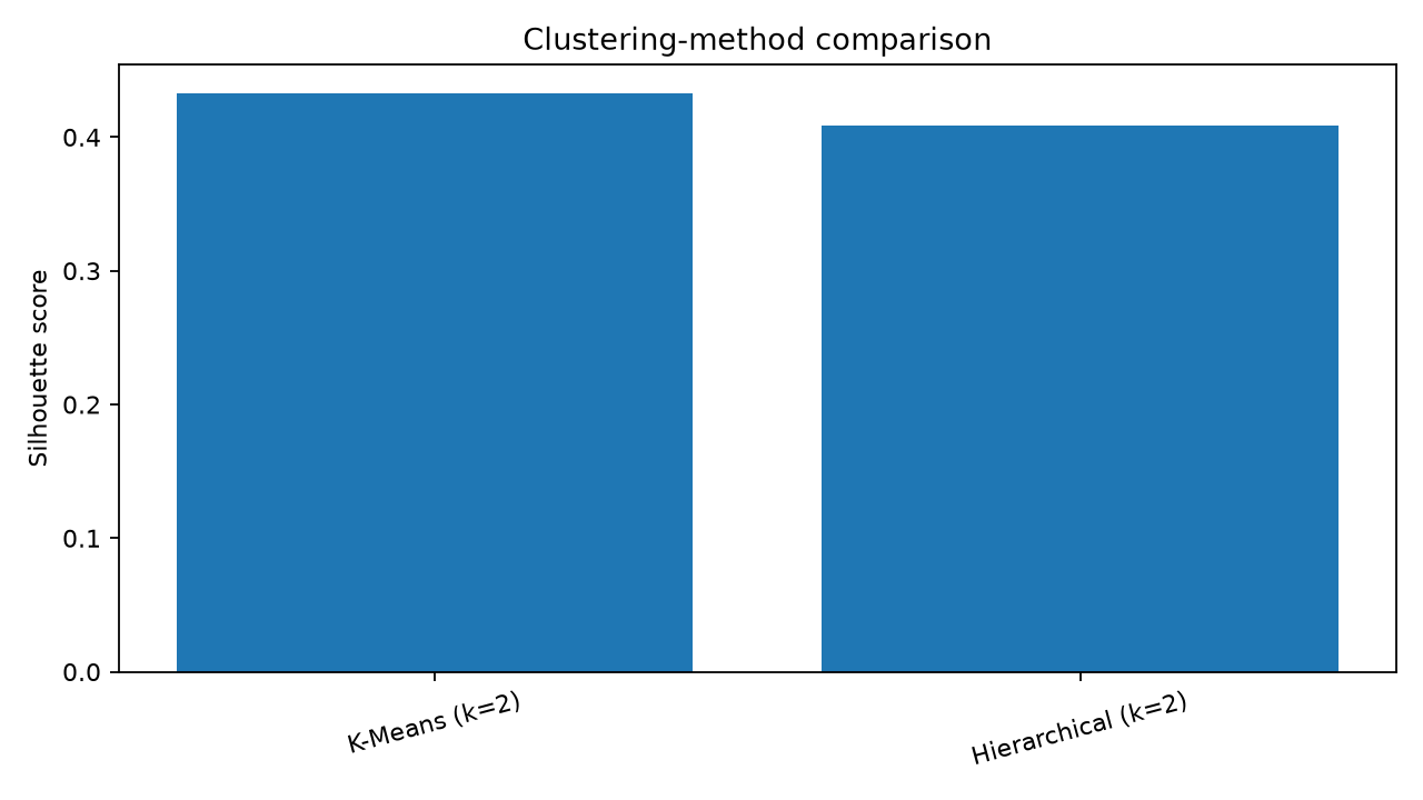
Step 9: Compare three different ideas about what a cluster is
kmeans = KMeans(n_clusters=selected_k, n_init=30, random_state=42)
kmeans_labels = kmeans.fit_predict(matrix)

hierarchical = AgglomerativeClustering(n_clusters=selected_k)
hierarchical_labels = hierarchical.fit_predict(matrix)

dbscan = DBSCAN(eps=0.65, min_samples=8)
dbscan_labels = dbscan.fit_predict(matrix)Real clustering-method comparison
Check before continuing
Step 10: Project three RFM dimensions into two so humans can inspect the result
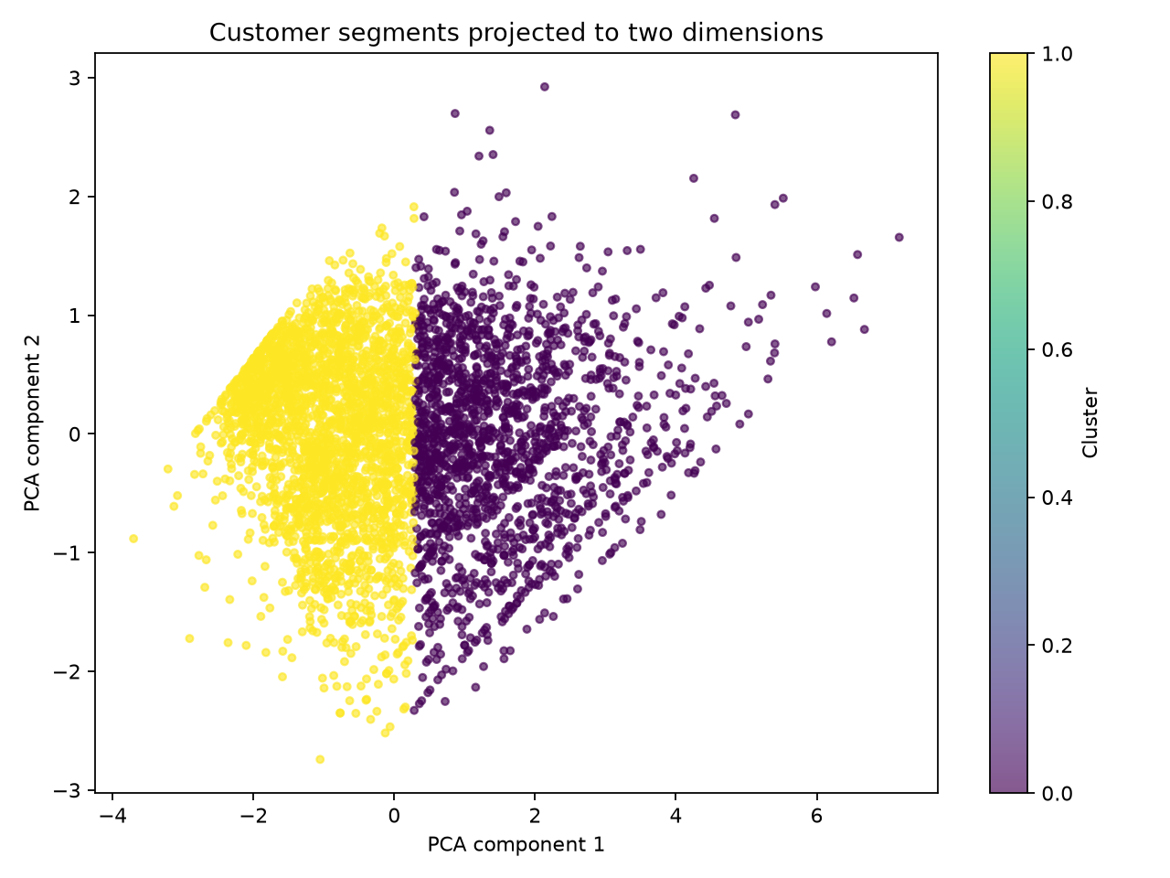
Two-dimensional view of the customer clusters
Check before continuing
Step 11: Translate numeric cluster IDs into understandable customer profiles
Why the segment names differ
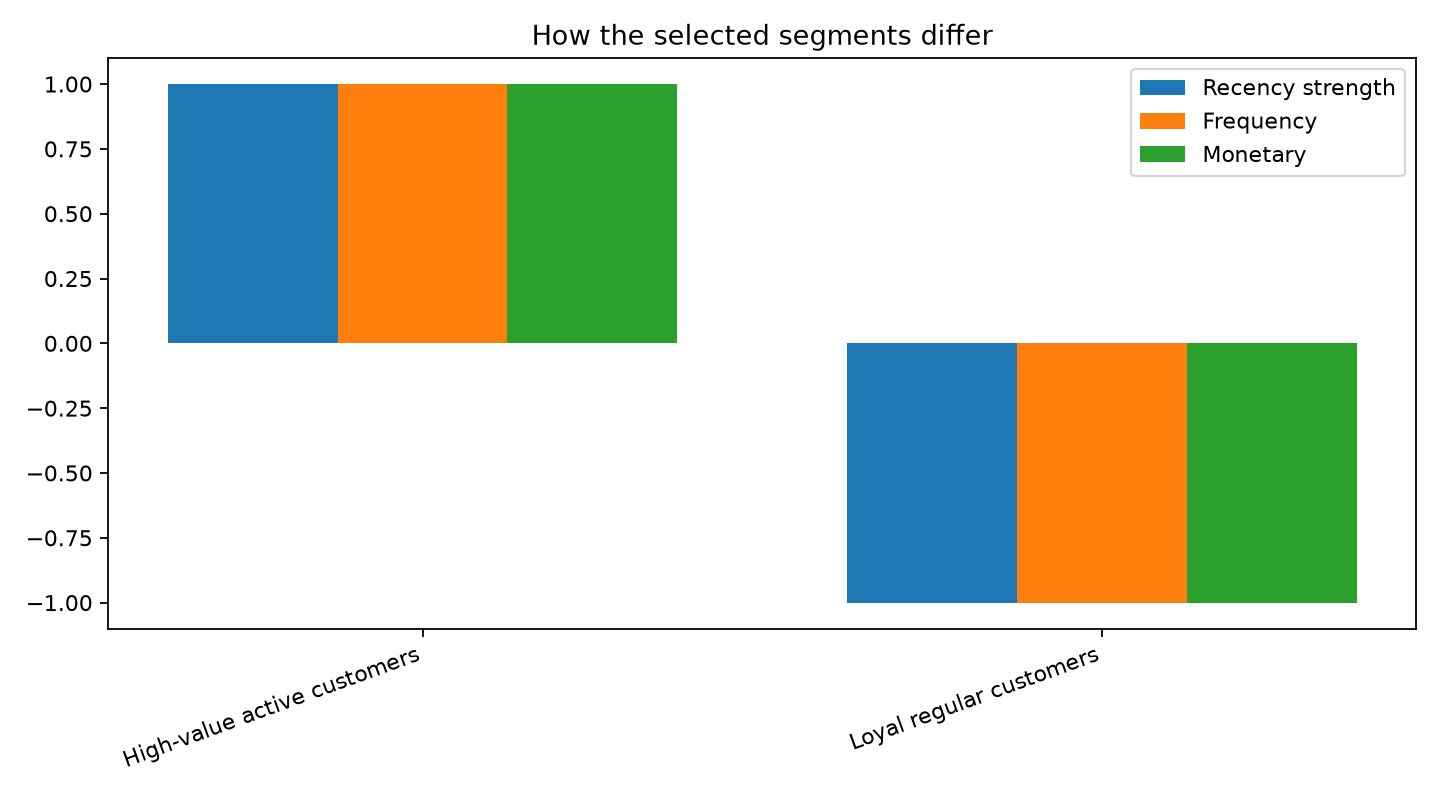
This two-cluster answer is what this dataset and these three RFM features support under the verified selection rule. If a business needs finer campaign groups, that is a new modeling requirement—not permission to arbitrarily force more clusters and call them “better”.
Check before continuing
Step 12: Assemble the complete verified segmentation engine
Open complete src/build_segments.py
Use the complete source only after understanding the earlier blocks.
"""Build RFM customer segments from the UCI Online Retail dataset."""

from __future__ import annotations

from pathlib import Path
import json

import joblib
import matplotlib.pyplot as plt
import numpy as np
import pandas as pd
from sklearn.cluster import AgglomerativeClustering, DBSCAN, KMeans
from sklearn.decomposition import PCA
from sklearn.metrics import silhouette_score
from sklearn.preprocessing import StandardScaler

ROOT = Path(__file__).resolve().parents[1]
DATA_PATH = ROOT / "data" / "online_retail.parquet"
MODEL_DIR = ROOT / "models"
OUTPUT_DIR = ROOT / "outputs"
RANDOM_STATE = 42
RFM_COLUMNS = ["recency_days", "frequency_orders", "monetary_value"]


def load_transactions() -> pd.DataFrame:
    if not DATA_PATH.is_file():
        raise FileNotFoundError(
            "Dataset is missing. Run python download_data.py first."
        )
    frame = pd.read_parquet(DATA_PATH).copy()
    frame["InvoiceNo"] = frame["InvoiceNo"].astype(str)
    frame["InvoiceDate"] = pd.to_datetime(frame["InvoiceDate"], errors="raise")
    frame["CustomerID"] = pd.to_numeric(frame["CustomerID"], errors="coerce")
    return frame


def clean_transactions(frame: pd.DataFrame) -> pd.DataFrame:
    cleaned = frame.loc[
        frame["CustomerID"].notna()
        & ~frame["InvoiceNo"].str.upper().str.startswith("C")
        & (frame["Quantity"] > 0)
        & (frame["UnitPrice"] > 0)
    ].copy()
    cleaned["CustomerID"] = cleaned["CustomerID"].astype(int).astype(str)
    cleaned["revenue"] = cleaned["Quantity"].astype(float) * cleaned["UnitPrice"].astype(float)
    return cleaned


def build_rfm(cleaned: pd.DataFrame) -> tuple[pd.DataFrame, pd.Timestamp]:
    snapshot = cleaned["InvoiceDate"].max().normalize() + pd.Timedelta(days=1)
    rfm = (
        cleaned.groupby("CustomerID", as_index=False)
        .agg(
            last_purchase=("InvoiceDate", "max"),
            frequency_orders=("InvoiceNo", "nunique"),
            monetary_value=("revenue", "sum"),
            items_bought=("Quantity", "sum"),
        )
    )
    rfm["recency_days"] = (
        snapshot - rfm["last_purchase"].dt.normalize()
    ).dt.days.astype(int)
    rfm["average_order_value"] = (
        rfm["monetary_value"] / rfm["frequency_orders"]
    )
    rfm = rfm[
        [
            "CustomerID",
            "recency_days",
            "frequency_orders",
            "monetary_value",
            "items_bought",
            "average_order_value",
        ]
    ].copy()
    return rfm, snapshot


def transform_rfm(rfm: pd.DataFrame) -> tuple[StandardScaler, np.ndarray]:
    # log1p reduces the extreme right skew while keeping zero-safe arithmetic.
    logged = np.log1p(rfm[RFM_COLUMNS].astype(float))
    scaler = StandardScaler()
    matrix = scaler.fit_transform(logged)
    return scaler, matrix


def compare_kmeans(matrix: np.ndarray) -> pd.DataFrame:
    rows = []
    sample_size = min(5000, len(matrix))
    for k in range(2, 9):
        model = KMeans(
            n_clusters=k,
            n_init=20,
            random_state=RANDOM_STATE,
        )
        labels = model.fit_predict(matrix)
        silhouette = silhouette_score(
            matrix,
            labels,
            sample_size=sample_size,
            random_state=RANDOM_STATE,
        )
        rows.append(
            {
                "k": k,
                "inertia": float(model.inertia_),
                "silhouette": float(silhouette),
            }
        )
    return pd.DataFrame(rows)


def safe_silhouette(matrix: np.ndarray, labels: np.ndarray) -> float | None:
    mask = labels != -1
    unique = np.unique(labels[mask])
    if len(unique) < 2 or int(mask.sum()) < 3:
        return None
    return float(
        silhouette_score(
            matrix[mask],
            labels[mask],
            sample_size=min(5000, int(mask.sum())),
            random_state=RANDOM_STATE,
        )
    )


def build_segment_names(
    rfm: pd.DataFrame,
    labels: np.ndarray,
) -> tuple[pd.DataFrame, dict[int, str]]:
    profiled = rfm.copy()
    profiled["cluster"] = labels
    profiles = (
        profiled.groupby("cluster")
        .agg(
            customers=("CustomerID", "count"),
            recency_days=("recency_days", "mean"),
            frequency_orders=("frequency_orders", "mean"),
            monetary_value=("monetary_value", "mean"),
            average_order_value=("average_order_value", "mean"),
        )
        .reset_index()
    )

    z = profiles[["recency_days", "frequency_orders", "monetary_value"]].copy()
    for column in z:
        std = float(z[column].std(ddof=0))
        if std == 0:
            z[column] = 0.0
        else:
            z[column] = (z[column] - z[column].mean()) / std
    profiles["value_score"] = (
        -z["recency_days"] + z["frequency_orders"] + z["monetary_value"]
    )

    ordered = profiles.sort_values("value_score", ascending=False)["cluster"].tolist()
    palette = [
        "High-value active customers",
        "Loyal regular customers",
        "Growing customers",
        "Occasional customers",
        "Low-engagement customers",
        "At-risk customers",
        "Dormant customers",
        "Long-tail customers",
    ]
    names = {
        int(cluster): palette[min(index, len(palette) - 1)]
        for index, cluster in enumerate(ordered)
    }
    profiles["segment_name"] = profiles["cluster"].map(names)
    return profiles.sort_values("value_score", ascending=False), names


def save_figures(
    rfm: pd.DataFrame,
    matrix: np.ndarray,
    labels: np.ndarray,
    k_table: pd.DataFrame,
    profiles: pd.DataFrame,
    method_rows: list[dict],
) -> None:
    OUTPUT_DIR.mkdir(exist_ok=True)

    fig, axes = plt.subplots(1, 3, figsize=(13, 4))
    for ax, column, title in zip(
        axes,
        RFM_COLUMNS,
        ["Recency", "Frequency", "Monetary value"],
    ):
        ax.hist(rfm[column], bins=40)
        ax.set_title(title)
        ax.set_xlabel(column)
        ax.set_ylabel("Customers")
    fig.tight_layout()
    fig.savefig(OUTPUT_DIR / "rfm_distributions.png", dpi=160)
    plt.close(fig)

    fig, ax1 = plt.subplots(figsize=(8, 5))
    ax1.plot(k_table["k"], k_table["silhouette"], marker="o")
    ax1.set_xlabel("Number of K-Means clusters (k)")
    ax1.set_ylabel("Silhouette score")
    ax1.set_title("Choose k using separation, not guesswork")
    fig.tight_layout()
    fig.savefig(OUTPUT_DIR / "k_selection.png", dpi=160)
    plt.close(fig)

    pca = PCA(n_components=2, random_state=RANDOM_STATE)
    coords = pca.fit_transform(matrix)
    fig, ax = plt.subplots(figsize=(8, 6))
    scatter = ax.scatter(coords[:, 0], coords[:, 1], c=labels, s=12, alpha=0.65)
    ax.set_xlabel("PCA component 1")
    ax.set_ylabel("PCA component 2")
    ax.set_title("Customer segments projected to two dimensions")
    fig.colorbar(scatter, ax=ax, label="Cluster")
    fig.tight_layout()
    fig.savefig(OUTPUT_DIR / "pca_segments.png", dpi=160)
    plt.close(fig)

    profile_plot = profiles.sort_values("value_score", ascending=False)
    fig, ax = plt.subplots(figsize=(9, 5))
    x = np.arange(len(profile_plot))
    width = 0.25
    standardized = profile_plot[
        ["recency_days", "frequency_orders", "monetary_value"]
    ].copy()
    for column in standardized:
        std = float(standardized[column].std(ddof=0))
        standardized[column] = (
            0.0
            if std == 0
            else (standardized[column] - standardized[column].mean()) / std
        )
    ax.bar(x - width, -standardized["recency_days"], width, label="Recency strength")
    ax.bar(x, standardized["frequency_orders"], width, label="Frequency")
    ax.bar(x + width, standardized["monetary_value"], width, label="Monetary")
    ax.set_xticks(x)
    ax.set_xticklabels(profile_plot["segment_name"], rotation=20, ha="right")
    ax.set_title("How the selected segments differ")
    ax.legend()
    fig.tight_layout()
    fig.savefig(OUTPUT_DIR / "cluster_profiles.png", dpi=160)
    plt.close(fig)

    methods = pd.DataFrame(method_rows)
    valid = methods.dropna(subset=["silhouette"])
    fig, ax = plt.subplots(figsize=(8, 4.5))
    ax.bar(valid["method"], valid["silhouette"])
    ax.set_ylabel("Silhouette score")
    ax.set_title("Clustering-method comparison")
    ax.tick_params(axis="x", rotation=15)
    fig.tight_layout()
    fig.savefig(OUTPUT_DIR / "method_comparison.png", dpi=160)
    plt.close(fig)


def main() -> None:
    MODEL_DIR.mkdir(exist_ok=True)
    OUTPUT_DIR.mkdir(exist_ok=True)

    raw = load_transactions()
    cleaned = clean_transactions(raw)
    rfm, snapshot = build_rfm(cleaned)
    scaler, matrix = transform_rfm(rfm)

    k_table = compare_kmeans(matrix)
    selected_k = int(
        k_table.sort_values(
            ["silhouette", "k"],
            ascending=[False, True],
        ).iloc[0]["k"]
    )

    kmeans = KMeans(
        n_clusters=selected_k,
        n_init=30,
        random_state=RANDOM_STATE,
    )
    kmeans_labels = kmeans.fit_predict(matrix)
    kmeans_silhouette = float(
        silhouette_score(
            matrix,
            kmeans_labels,
            sample_size=min(5000, len(matrix)),
            random_state=RANDOM_STATE,
        )
    )

    hierarchical = AgglomerativeClustering(n_clusters=selected_k)
    hierarchical_labels = hierarchical.fit_predict(matrix)
    hierarchical_silhouette = float(
        silhouette_score(
            matrix,
            hierarchical_labels,
            sample_size=min(5000, len(matrix)),
            random_state=RANDOM_STATE,
        )
    )

    dbscan = DBSCAN(eps=0.65, min_samples=8)
    dbscan_labels = dbscan.fit_predict(matrix)
    dbscan_silhouette = safe_silhouette(matrix, dbscan_labels)

    profiles, names = build_segment_names(rfm, kmeans_labels)
    segmented = rfm.copy()
    segmented["cluster"] = kmeans_labels
    segmented["segment_name"] = segmented["cluster"].map(names)

    method_rows = [
        {
            "method": f"K-Means (k={selected_k})",
            "silhouette": kmeans_silhouette,
            "clusters": selected_k,
            "noise_customers": 0,
        },
        {
            "method": f"Hierarchical (k={selected_k})",
            "silhouette": hierarchical_silhouette,
            "clusters": selected_k,
            "noise_customers": 0,
        },
        {
            "method": "DBSCAN",
            "silhouette": dbscan_silhouette,
            "clusters": int(len(set(dbscan_labels)) - (1 if -1 in dbscan_labels else 0)),
            "noise_customers": int((dbscan_labels == -1).sum()),
        },
    ]

    k_table.to_csv(OUTPUT_DIR / "kmeans_k_comparison.csv", index=False)
    pd.DataFrame(method_rows).to_csv(
        OUTPUT_DIR / "clustering_method_comparison.csv",
        index=False,
    )
    profiles.to_csv(OUTPUT_DIR / "segment_profiles.csv", index=False)
    segmented.to_csv(OUTPUT_DIR / "customer_segments.csv", index=False)

    bundle = {
        "scaler": scaler,
        "kmeans": kmeans,
        "rfm_columns": RFM_COLUMNS,
        "segment_names": names,
        "segment_profiles": profiles,
        "snapshot_date": str(snapshot.date()),
        "selected_k": selected_k,
    }
    joblib.dump(bundle, MODEL_DIR / "customer_segmenter.joblib")
    reloaded = joblib.load(MODEL_DIR / "customer_segmenter.joblib")

    example = pd.DataFrame(
        [{"recency_days": 30, "frequency_orders": 5, "monetary_value": 800.0}]
    )
    example_matrix = reloaded["scaler"].transform(np.log1p(example[RFM_COLUMNS]))
    example_cluster = int(reloaded["kmeans"].predict(example_matrix)[0])

    metrics = {
        "raw_rows": int(len(raw)),
        "clean_purchase_rows": int(len(cleaned)),
        "customers": int(len(rfm)),
        "snapshot_date": str(snapshot.date()),
        "selected_k": selected_k,
        "kmeans_silhouette": kmeans_silhouette,
        "hierarchical_silhouette": hierarchical_silhouette,
        "dbscan_silhouette": dbscan_silhouette,
        "dbscan_noise_customers": int((dbscan_labels == -1).sum()),
        "example_cluster": example_cluster,
        "example_segment": names[example_cluster],
    }
    (OUTPUT_DIR / "metrics.json").write_text(
        json.dumps(metrics, indent=2) + "\n",
        encoding="utf-8",
    )

    save_figures(
        rfm,
        matrix,
        kmeans_labels,
        k_table,
        profiles,
        method_rows,
    )

    print("Customer segmentation build completed.")
    print(json.dumps(metrics, indent=2))
    print("\nSelected K-Means profiles:")
    print(
        profiles[
            [
                "cluster",
                "segment_name",
                "customers",
                "recency_days",
                "frequency_orders",
                "monetary_value",
            ]
        ].to_string(index=False)
    )


if __name__ == "__main__":
    main()
python src/build_segments.pyraw_rows: 541909
clean_purchase_rows: 397884
customers: 4338
selected_k: 2
kmeans_silhouette: 0.432624
hierarchical_silhouette: 0.408629
example_segment: High-value active customersCheck before continuing
Step 13: Save the scaler and K-Means model together
The Joblib bundle stores the fitted scaler, fitted K-Means model, RFM feature order, chosen k, snapshot date, segment names and profiles. That avoids the common mistake of scaling new customers differently from the historical customers.
Check before continuing
Step 14: Build the Streamlit customer-segmentation app
Open complete app.py
"""Run from the project root with: python -m streamlit run app.py"""

from pathlib import Path

import joblib
import numpy as np
import pandas as pd
import streamlit as st

ROOT = Path(__file__).resolve().parent
MODEL_PATH = ROOT / "models" / "customer_segmenter.joblib"
RFM_COLUMNS = ["recency_days", "frequency_orders", "monetary_value"]

st.set_page_config(
    page_title="Customer Segmentation",
    page_icon="🛍️",
    layout="wide",
)
st.title("How Amazon Knows What Kind of Customer You Are")
st.caption(
    "Educational customer-segmentation project using UCI Online Retail data • "
    "not Amazon data or Amazon's production algorithm"
)

if not MODEL_PATH.is_file():
    st.error("The saved customer-segmentation artifact is missing.")
    st.code(
        "python download_data.py\npython src/build_segments.py",
        language="powershell",
    )
    st.stop()


@st.cache_resource
def load_bundle(modified_ns: int):
    return joblib.load(MODEL_PATH)


bundle = load_bundle(MODEL_PATH.stat().st_mtime_ns)
profiles = bundle["segment_profiles"].copy()

st.info(
    "RFM means Recency, Frequency and Monetary value. The model groups customers "
    "by shopping behaviour without a pre-existing target label."
)

left, right = st.columns([1, 1.3])

with left:
    st.subheader("Try a customer profile")
    recency = st.number_input(
        "Days since last purchase",
        min_value=0,
        max_value=800,
        value=30,
        step=1,
    )
    frequency = st.number_input(
        "Number of completed orders",
        min_value=1,
        max_value=500,
        value=5,
        step=1,
    )
    monetary = st.number_input(
        "Total historical spend (£)",
        min_value=0.01,
        max_value=500000.0,
        value=800.0,
        step=50.0,
    )

    if st.button("Find customer segment", type="primary", use_container_width=True):
        row = pd.DataFrame(
            [{
                "recency_days": float(recency),
                "frequency_orders": float(frequency),
                "monetary_value": float(monetary),
            }]
        )
        transformed = bundle["scaler"].transform(np.log1p(row[RFM_COLUMNS]))
        cluster = int(bundle["kmeans"].predict(transformed)[0])
        segment = bundle["segment_names"][cluster]
        st.success(f"Assigned segment: {segment}")
        st.write(f"Cluster ID: {cluster}")
        st.caption(
            "The name is an educational interpretation of that cluster's average RFM profile."
        )

with right:
    st.subheader("Verified segment profiles")
    display = profiles[
        [
            "segment_name",
            "customers",
            "recency_days",
            "frequency_orders",
            "monetary_value",
        ]
    ].copy()
    display.columns = [
        "Segment",
        "Customers",
        "Avg recency (days)",
        "Avg orders",
        "Avg spend (£)",
    ]
    st.dataframe(display, hide_index=True, use_container_width=True)
    st.caption(
        f"Selected K-Means clusters: {bundle['selected_k']} • "
        f"RFM snapshot date: {bundle['snapshot_date']}"
    )

st.divider()
st.caption(
    "This project demonstrates RFM clustering on a public UK online-retail dataset. "
    "Real companies may use many more behavioural, product, demographic and real-time signals."
)
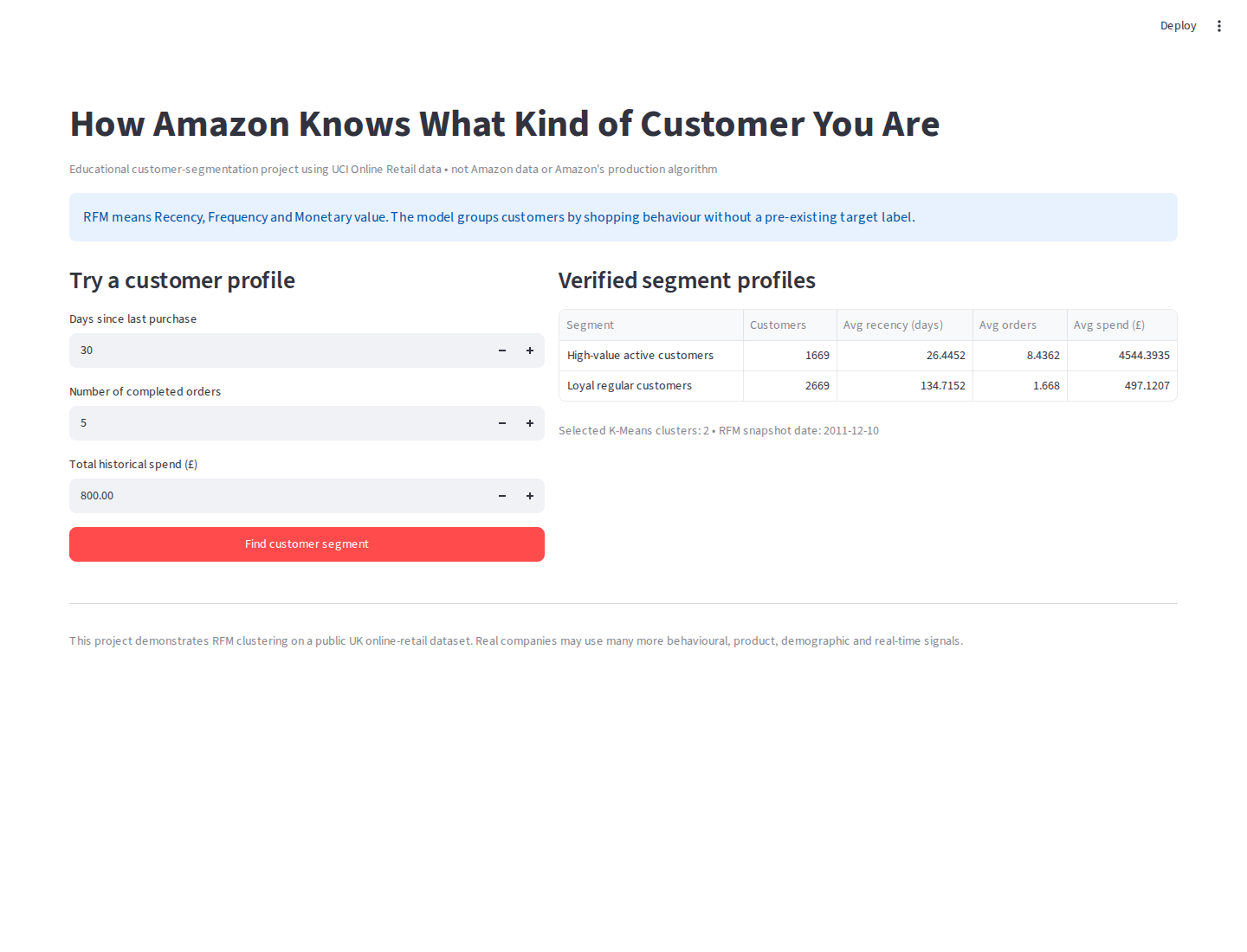
python -m streamlit run app.pyReal app before assignment
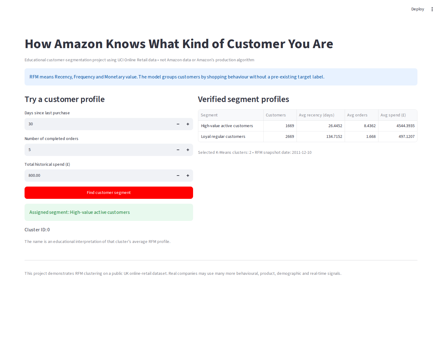
Real saved-model assignment
Check before continuing
Step 15: Prove the project works with automated tests
Open tests/test_customer_segmentation.py
from pathlib import Path
import importlib.util

import joblib
import numpy as np
import pandas as pd

ROOT = Path(__file__).resolve().parents[1]
MODEL_PATH = ROOT / "models" / "customer_segmenter.joblib"

spec = importlib.util.spec_from_file_location(
    "customer_segments",
    ROOT / "src" / "build_segments.py",
)
core = importlib.util.module_from_spec(spec)
spec.loader.exec_module(core)


def test_downloaded_dataset_contract():
    frame = core.load_transactions()
    assert len(frame) == 541_909
    assert {
        "InvoiceNo",
        "Quantity",
        "InvoiceDate",
        "UnitPrice",
        "CustomerID",
        "Country",
    }.issubset(frame.columns)


def test_cleaning_removes_cancellations_and_invalid_purchases():
    cleaned = core.clean_transactions(core.load_transactions())
    assert cleaned["CustomerID"].notna().all()
    assert (cleaned["Quantity"] > 0).all()
    assert (cleaned["UnitPrice"] > 0).all()
    assert not cleaned["InvoiceNo"].str.upper().str.startswith("C").any()


def test_rfm_has_positive_business_features():
    cleaned = core.clean_transactions(core.load_transactions())
    rfm, snapshot = core.build_rfm(cleaned)
    assert len(rfm) > 4_000
    assert (rfm["recency_days"] >= 1).all()
    assert (rfm["frequency_orders"] >= 1).all()
    assert (rfm["monetary_value"] > 0).all()
    assert snapshot > cleaned["InvoiceDate"].max()


def test_saved_bundle_and_profiles_exist():
    assert MODEL_PATH.is_file()
    bundle = joblib.load(MODEL_PATH)
    assert 2 <= int(bundle["selected_k"]) <= 8
    assert len(bundle["segment_names"]) == int(bundle["selected_k"])
    assert len(bundle["segment_profiles"]) == int(bundle["selected_k"])


def test_example_prediction_is_deterministic():
    bundle = joblib.load(MODEL_PATH)
    row = pd.DataFrame(
        [{"recency_days": 30.0, "frequency_orders": 5.0, "monetary_value": 800.0}]
    )
    transformed = bundle["scaler"].transform(
        np.log1p(row[bundle["rfm_columns"]])
    )
    first = int(bundle["kmeans"].predict(transformed)[0])
    second = int(bundle["kmeans"].predict(transformed)[0])
    assert first == second
    assert first in bundle["segment_names"]


def test_required_outputs_exist():
    for name in [
        "metrics.json",
        "kmeans_k_comparison.csv",
        "clustering_method_comparison.csv",
        "segment_profiles.csv",
        "customer_segments.csv",
        "rfm_distributions.png",
        "k_selection.png",
        "pca_segments.png",
        "cluster_profiles.png",
        "method_comparison.png",
    ]:
        assert (ROOT / "outputs" / name).is_file(), name
pytest -q
......
6 passed in 2.14s
Check before continuing
Step 16: Understand the complete project folder
├── data/ # downloaded locally; not committed
├── models/customer_segmenter.joblib # generated artifact
├── outputs/ # metrics, CSVs, figures, screenshots
├── scripts/capture_app_screenshots.py
├── src/build_segments.py
├── tests/test_customer_segmentation.py
├── app.py
├── download_data.py
├── requirements.txt
└── README.md
Check before continuing
Troubleshooting checkpoints
Parquet says it cannot convert an invoice such as C536379: invoice IDs mix numeric-looking values and cancellation codes. Keep identifiers as strings before Parquet export.
One feature dominates the clusters: verify that log transformation and StandardScaler are applied to all three RFM features.
DBSCAN gives mostly one cluster or lots of noise: density methods are sensitive to eps and min_samples. Do not force a misleading silhouette score when fewer than two non-noise clusters exist.
Your cluster numbers change meaning: cluster IDs are arbitrary. Interpret clusters from their measured RFM profiles, never from the number 0/1/2 itself.
How to explain this project in an interview
Why is this unsupervised learning?
There is no target label telling us the correct customer segment. We discover structure from RFM behaviour.
Why clean before aggregation?
Cancellations, returns and unknown customers would distort revenue, order counts and recency.
Why log-transform and scale?
RFM features are skewed and measured on very different numeric ranges; distance-based clustering is sensitive to that.
Why silhouette rather than only the elbow method?
Silhouette explicitly compares within-cluster cohesion with separation from neighboring clusters. We still treat it as evidence, not business truth.
Why compare DBSCAN?
It represents a different density-based idea of a cluster and can identify noise instead of forcing every customer into a centroid-based group.
Why is PCA not the clustering algorithm here?
PCA is used to project the transformed three-dimensional RFM space into two dimensions for visualization.