FREE · VERIFIED BUILDBeginnerWindows-first instructions

What Is This House Really Worth? Build a House Price Predictor

Start with an empty folder. Download the real Ames Housing dataset, train five regression models, compare them correctly, tune the winner, save it, and run your own house-price prediction app in a browser.

Real Streamlit House Price Predictor app created and tested for this handbook

This is the actual application built for this handbook. The screenshot above was captured automatically from the working Streamlit application after the complete training pipeline passed. It is not a mock-up or generated illustration.

What you will build

A browser app where a user enters property details such as living area, bathrooms, garage size, year built, neighborhood and quality. A trained model then estimates the historical sale price.

What you need before starting

Basic laptop operation: opening a browser, creating folders, clicking menus and typing text. You do not need previous Python or machine-learning experience.

Topics covered

These are the ideas you will learn while building.

Machine LearningSupervised LearningRegressionFeature EngineeringMissing-Value ImputationCategorical EncodingFeature ScalingScikit-learn PipelinesLinear RegressionRidgeLassoRandom ForestXGBoostCross-ValidationHyperparameter TuningMAERMSER²Model PersistenceInferenceDeployment

Tools you will actually use

Algorithms are not listed as tools. These are the applications and libraries used in the real build.

PythonVS CodeOpenMLPandasNumPyMatplotlibScikit-learnXGBoostJoblibStreamlitPytestGitGitHub

Verified result from the build used for this handbook

Winner

XGBoost

Holdout MAE

$15,670

Holdout RMSE

$23,792

Holdout R²

0.929

These are real values from the verified project run. Your exact numbers should be the same when using the same dataset, package versions and random seed, although small library/platform differences can occasionally create tiny numerical differences.

How the complete system fits together

Before touching the code, understand the journey. The project has two connected halves: training, where we learn a model from historical sales, and inference, where the saved model receives one new property and returns an estimated price.

Training path

OpenML → download_data.py → Ames dataset → train_model.py → feature engineering → preprocessing → 5-fold model comparison → XGBoost tuning → untouched holdout evaluation →house_price_pipeline.joblib + metrics + chart.

Prediction path

User enters property details in Streamlit → app.py builds the same feature shape → saved pipeline applies the preprocessing learned during training → XGBoost predicts → the browser displays the estimated historical sale price.

The important design idea is that the app does not retrain the model. Training happens once, the fitted pipeline is saved, and the application only loads that artifact for prediction.

Install Python on Windows

Open Chrome, Edge or another browser. Go to the official Python downloads for Windows page.

Use a current 64-bit Python 3 release supported by the packages in this project. This project is continuously verified with Python 3.12 in automation. If you already have Python 3.12 installed, keep it.

Download the Windows installer/install manager from Python.org.
Run the downloaded installer.
If your installer offers an option to make Python available from the command line or add it to PATH, enable it.
Finish installation.
Open the Windows Start menu, type PowerShell, and open Windows PowerShell.
Type python --version and press Enter.

PowerShellpowershellRunnable

python --version

If Windows says Python is not recognized, close PowerShell, reopen it once, and try again. If it still fails, rerun the Python installer and enable command-line/PATH integration.

Check before continuing: PowerShell prints a Python version when you type python --version.

Install VS Code and the Python extension

Go to the official Visual Studio Code download page, download the Windows installer and install it using the default options.

Open VS Code.
Look at the vertical icon bar on the far left.
Click the Extensions icon. It looks like four small blocks.
Type Python in the search box.
Choose the extension named Python published by Microsoft.
Click Install.

We will use VS Code as the place where you create folders, create files, paste code and open the terminal.

Check before continuing: VS Code opens and the Extensions panel shows the Microsoft Python extension as installed.

Create the project folder and open it in VS Code

On your Desktop, create a folder named house-price-predictor.

Open VS Code.
Click File → Open Folder....
Select the new house-price-predictor folder.
If VS Code asks whether you trust the folder, choose the option appropriate for a folder you just created yourself.

In VS Code, the Explorer is the left panel that shows your files. The terminal is a text area where we type commands and press Enter to run them.

Open Terminal → New Terminal. A terminal panel should appear at the bottom of VS Code.

Check before continuing: The VS Code Explorer shows the house-price-predictor folder.

Create the folders the project needs

Click inside the VS Code terminal, paste the commands below and press Enter.

Create the project structurepowershellRunnable

mkdir house-price-predictor
cd house-price-predictor
mkdir data
mkdir models
mkdir outputs
mkdir src
mkdir tests

If you opened the folder itself in VS Code already, you may already be inside house-price-predictor. In that case, do not create a second nested folder. Create only data, models,outputs, src and tests using Explorer's New Folder button.

house-price-predictor/
├── data/
├── models/
├── outputs/
├── src/
└── tests/

Check before continuing: Explorer shows data, models, outputs, src and tests.

Create and activate a virtual environment

A virtual environment is a private Python environment for this project. It prevents this project's package versions from interfering with packages used by another project.

Make sure the terminal is inside the project root, then run:

Create and activate .venvpowershellRunnable

python -m venv .venv
.venv\Scripts\Activate.ps1
python --version
python -m pip --version

If PowerShell blocks Activate.ps1, run Set-ExecutionPolicy -Scope Process -ExecutionPolicy Bypass in that same terminal and activate again. The -Scope Process choice applies only to that PowerShell process.

Check before continuing: The terminal prompt begins with (.venv), and python --version works.

Create requirements.txt and install the exact packages

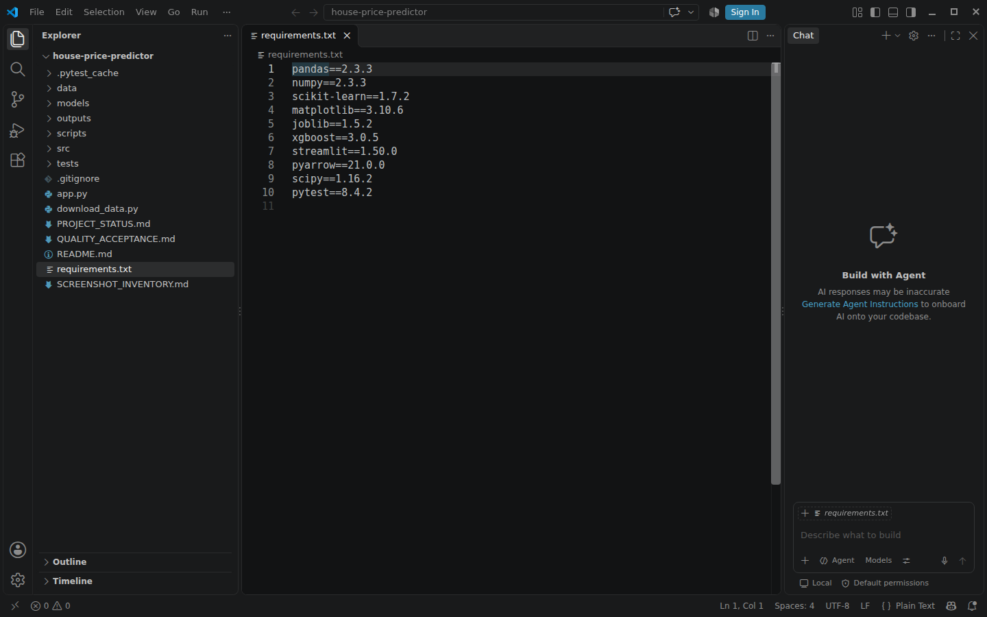
In Explorer, move your mouse over the project name and click the New File icon. Name the filerequirements.txt. Paste the complete content below and press Ctrl+S to save.

requirements.txttextConfiguration

pandas==2.3.3
numpy==2.3.3
scikit-learn==1.7.2
matplotlib==3.10.6
joblib==1.5.2
xgboost==3.0.5
streamlit==1.50.0
pyarrow==21.0.0
scipy==1.16.2
pytest==8.4.2

Real Visual Studio Code window showing the verified requirements.txt file for the House Price Predictor project — Real screenshot captured from the project in Visual Studio Code. Your desktop VS Code may use a different theme, but the filename and contents should match.

Return to the terminal and run:

Install the project dependenciespowershellRunnable

python -m pip install --upgrade pip
pip install -r requirements.txt

What just happened? pip downloaded the exact versions of Pandas, NumPy, scikit-learn, XGBoost, Streamlit and the other libraries that our verified build used.

Check before continuing: The installation finishes without a red ERROR line.

Create the official Ames Housing dataset downloader

We are using the Ames Housing dataset. It contains historical residential property sales from Ames, Iowa and was created for data-science education. The prediction target is the property's sale price.

Open the official OpenML Ames Housing page. You do not need to manually rename or move a downloaded CSV in this project. We will create a small Python downloader that retrieves the dataset from OpenML and stores it in the correct folder automatically.

In the project root create a file named download_data.py. Paste all of this code, then save it:

download_data.pypythonRunnable

from __future__ import annotations

import io
import sys
import urllib.request
from pathlib import Path

import pandas as pd
from scipy.io import arff

PROJECT_ROOT = Path(__file__).resolve().parent
DATA_DIR = PROJECT_ROOT / "data"
OUTPUT_PATH = DATA_DIR / "ames_housing.parquet"

OPENML_DATASET_PAGE = "https://www.openml.org/search?id=43926&sort=runs&type=data"
OPENML_PARQUET_URL = "https://data.openml.org/datasets/0004/43926/dataset_43926.pq"
OPENML_ARFF_URL = "https://openml.org/data/v1/download/22102974/ames_housing.arff"


def _decode_bytes_columns(frame: pd.DataFrame) -> pd.DataFrame:
    for column in frame.columns:
        if frame[column].dtype == object:
            frame[column] = frame[column].map(
                lambda value: value.decode("utf-8") if isinstance(value, bytes) else value
            )
    return frame


def download_dataset() -> Path:
    DATA_DIR.mkdir(parents=True, exist_ok=True)

    print("Dataset: Ames Housing")
    print("Official OpenML page:", OPENML_DATASET_PAGE)
    print("Target: house sale price")
    print("Expected rows: 2,930")

    try:
        print("\nTrying the official OpenML parquet file...")
        frame = pd.read_parquet(OPENML_PARQUET_URL)
    except Exception as parquet_error:
        print("Parquet download failed:", parquet_error)
        print("Trying the official OpenML ARFF file instead...")
        try:
            with urllib.request.urlopen(OPENML_ARFF_URL, timeout=90) as response:
                raw_bytes = response.read()
            data, _meta = arff.loadarff(io.BytesIO(raw_bytes))
            frame = _decode_bytes_columns(pd.DataFrame(data))
        except Exception as arff_error:
            raise RuntimeError(
                "Could not download the Ames Housing dataset from OpenML. "
                "Check your internet connection and try again."
            ) from arff_error

    if len(frame) < 2900:
        raise RuntimeError(f"Dataset looks incomplete: only {len(frame)} rows were downloaded.")

    frame.to_parquet(OUTPUT_PATH, index=False)
    print(f"\nSaved {len(frame):,} rows and {len(frame.columns)} columns to:")
    print(OUTPUT_PATH)
    return OUTPUT_PATH


if __name__ == "__main__":
    try:
        download_dataset()
    except Exception as error:
        print(f"\nERROR: {error}", file=sys.stderr)
        raise

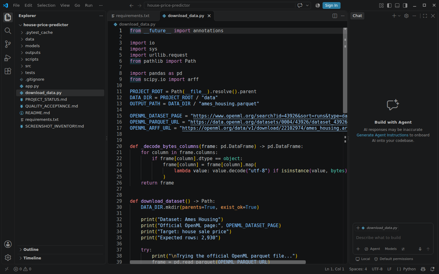
Real Visual Studio Code window showing download_data.py in the verified House Price Predictor project — This is the actual downloader file used by the verified build. Use the Copy button above rather than typing the program by hand.

Run it from the project root:

Download the real datasetpowershellRunnable

python download_data.py

Expected checkpoint outputtextOutput

Dataset: Ames Housing
Official OpenML page: https://www.openml.org/search?id=43926&sort=runs&type=data
Target: house sale price
Expected rows: 2,930

Trying the official OpenML parquet file...

Saved 2,930 rows and 81 columns to:
...\data\ames_housing.parquet

A row is one home sale. A column is one recorded property characteristic such as living area or garage capacity. The target is the value we want the model to predict.

Check before continuing: Running the downloader reports 2,930 rows and 81 columns and creates data/ames_housing.parquet.

Understand the features before training

We deliberately use a manageable subset of the 81 dataset columns so a beginner can understand what goes into the prediction instead of feeding every field into a black box.

Field	Meaning	Type
Gr_Liv_Area	Above-ground living area in square feet	numeric
Garage_Cars	How many cars fit in the garage	numeric
Total_Bsmt_SF	Total basement area	numeric
Year_Built	Year the home was originally built	numeric
Neighborhood	Neighborhood category	categorical
Kitchen_Qual	Kitchen quality label	categorical
Overall_Qual	Overall material/finish quality label	categorical
Sale_Price	The historical sale price we predict	target

Numeric data can be measured as numbers. Categorical data represents named groups. Machine-learning libraries ultimately need numbers, so the pipeline will convert categories to model-ready columns automatically.

Check before continuing: You can explain the difference between a feature and the target Sale_Price.

Create the complete training program

In Explorer open the src folder. Create train_model.py. This is the program that builds and evaluates the machine-learning system.

The program below is exactly the source used for the verified build. Do not type it manually line by line; use the Copy button, paste it into the file, and save.

src/train_model.py — complete verified training programpythonRunnable

from __future__ import annotations

import json
import re
from pathlib import Path

import joblib
import matplotlib.pyplot as plt
import numpy as np
import pandas as pd
from sklearn.compose import ColumnTransformer
from sklearn.ensemble import RandomForestRegressor
from sklearn.impute import SimpleImputer
from sklearn.linear_model import Lasso, LinearRegression, Ridge
from sklearn.metrics import mean_absolute_error, mean_squared_error, r2_score
from sklearn.model_selection import GridSearchCV, KFold, cross_validate, train_test_split
from sklearn.pipeline import Pipeline
from sklearn.preprocessing import OneHotEncoder, StandardScaler
from xgboost import XGBRegressor

PROJECT_ROOT = Path(__file__).resolve().parents[1]
DATA_PATH = PROJECT_ROOT / "data" / "ames_housing.parquet"
MODELS_DIR = PROJECT_ROOT / "models"
OUTPUTS_DIR = PROJECT_ROOT / "outputs"

RANDOM_STATE = 42

RAW_NUMERIC_FEATURES = [
    "gr_liv_area",
    "garage_cars",
    "garage_area",
    "total_bsmt_sf",
    "full_bath",
    "half_bath",
    "bedroom_abv_gr",
    "fireplaces",
    "year_built",
    "year_remod_add",
    "year_sold",
    "lot_area",
]
RAW_CATEGORICAL_FEATURES = [
    "neighborhood",
    "house_style",
    "kitchen_qual",
    "overall_qual",
]
MODEL_NUMERIC_FEATURES = [
    "gr_liv_area",
    "garage_cars",
    "garage_area",
    "total_bsmt_sf",
    "bedroom_abv_gr",
    "fireplaces",
    "lot_area",
    "house_age_at_sale",
    "years_since_remodel",
    "total_bathrooms",
]
MODEL_CATEGORICAL_FEATURES = RAW_CATEGORICAL_FEATURES
TARGET = "sale_price"


def normalize_column_name(name: str) -> str:
    value = str(name).strip()
    value = re.sub(r"([a-z0-9])([A-Z])", r"\1_\2", value)
    value = value.replace("/", "_")
    value = re.sub(r"[^A-Za-z0-9]+", "_", value)
    return value.strip("_").lower()


def normalize_columns(frame: pd.DataFrame) -> pd.DataFrame:
    normalized = frame.copy()
    normalized.columns = [normalize_column_name(column) for column in normalized.columns]
    return normalized


def build_model_frame(frame: pd.DataFrame) -> tuple[pd.DataFrame, pd.Series]:
    frame = normalize_columns(frame)

    required = set(RAW_NUMERIC_FEATURES + RAW_CATEGORICAL_FEATURES + [TARGET])
    missing = sorted(required.difference(frame.columns))
    if missing:
        raise KeyError(
            "The dataset does not contain the expected columns: " + ", ".join(missing)
        )

    working = frame[list(required)].copy()

    for column in RAW_NUMERIC_FEATURES + [TARGET]:
        working[column] = pd.to_numeric(working[column], errors="coerce")

    for column in RAW_CATEGORICAL_FEATURES:
        working[column] = working[column].astype("object")

    working["house_age_at_sale"] = working["year_sold"] - working["year_built"]
    working["years_since_remodel"] = working["year_sold"] - working["year_remod_add"]
    working["total_bathrooms"] = working["full_bath"] + (0.5 * working["half_bath"])

    features = working[MODEL_NUMERIC_FEATURES + MODEL_CATEGORICAL_FEATURES]
    target = working[TARGET]
    return features, target


def make_preprocessor(scale_numeric: bool) -> ColumnTransformer:
    numeric_steps = [("imputer", SimpleImputer(strategy="median"))]
    if scale_numeric:
        numeric_steps.append(("scaler", StandardScaler()))

    numeric_pipeline = Pipeline(numeric_steps)
    categorical_pipeline = Pipeline(
        [
            ("imputer", SimpleImputer(strategy="most_frequent")),
            (
                "onehot",
                OneHotEncoder(handle_unknown="ignore", sparse_output=False),
            ),
        ]
    )

    return ColumnTransformer(
        [
            ("numeric", numeric_pipeline, MODEL_NUMERIC_FEATURES),
            ("categorical", categorical_pipeline, MODEL_CATEGORICAL_FEATURES),
        ],
        remainder="drop",
    )


def make_pipeline(estimator, scale_numeric: bool) -> Pipeline:
    return Pipeline(
        [
            ("prepare", make_preprocessor(scale_numeric=scale_numeric)),
            ("model", estimator),
        ]
    )


def candidate_models() -> dict[str, Pipeline]:
    return {
        "Linear Regression": make_pipeline(LinearRegression(), scale_numeric=True),
        "Ridge": make_pipeline(Ridge(alpha=10.0), scale_numeric=True),
        "Lasso": make_pipeline(
            Lasso(alpha=250.0, max_iter=20000, random_state=RANDOM_STATE),
            scale_numeric=True,
        ),
        "Random Forest": make_pipeline(
            RandomForestRegressor(
                n_estimators=350,
                min_samples_leaf=1,
                random_state=RANDOM_STATE,
                n_jobs=-1,
            ),
            scale_numeric=False,
        ),
        "XGBoost": make_pipeline(
            XGBRegressor(
                objective="reg:squarederror",
                n_estimators=400,
                learning_rate=0.05,
                max_depth=3,
                subsample=0.9,
                colsample_bytree=0.9,
                random_state=RANDOM_STATE,
                n_jobs=2,
            ),
            scale_numeric=False,
        ),
    }


def compare_models(
    models: dict[str, Pipeline],
    X_train: pd.DataFrame,
    y_train: pd.Series,
) -> pd.DataFrame:
    cv = KFold(n_splits=5, shuffle=True, random_state=RANDOM_STATE)
    scoring = {
        "rmse": "neg_root_mean_squared_error",
        "mae": "neg_mean_absolute_error",
        "r2": "r2",
    }

    rows = []
    for name, pipeline in models.items():
        print(f"Cross-validating {name}...")
        scores = cross_validate(
            pipeline,
            X_train,
            y_train,
            cv=cv,
            scoring=scoring,
            n_jobs=1,
            error_score="raise",
        )
        rows.append(
            {
                "model": name,
                "cv_rmse_mean": -float(np.mean(scores["test_rmse"])),
                "cv_rmse_std": float(np.std(-scores["test_rmse"])),
                "cv_mae_mean": -float(np.mean(scores["test_mae"])),
                "cv_r2_mean": float(np.mean(scores["test_r2"])),
            }
        )

    return pd.DataFrame(rows).sort_values("cv_rmse_mean").reset_index(drop=True)


def tuning_grid(model_name: str) -> dict[str, list]:
    if model_name == "Ridge":
        return {"model__alpha": [0.1, 1.0, 10.0, 50.0, 100.0]}
    if model_name == "Lasso":
        return {"model__alpha": [50.0, 100.0, 250.0, 500.0, 1000.0]}
    if model_name == "Random Forest":
        return {
            "model__n_estimators": [300, 500],
            "model__max_features": ["sqrt", 0.8],
            "model__min_samples_leaf": [1, 2],
        }
    if model_name == "XGBoost":
        return {
            "model__n_estimators": [250, 450],
            "model__max_depth": [2, 3],
            "model__learning_rate": [0.03, 0.06],
        }
    return {}


def build_metadata(
    raw_frame: pd.DataFrame,
    winning_model: str,
    final_metrics: dict[str, float],
) -> dict:
    raw_frame = normalize_columns(raw_frame)

    numeric_defaults = {}
    for column in RAW_NUMERIC_FEATURES:
        series = pd.to_numeric(raw_frame[column], errors="coerce").dropna()
        numeric_defaults[column] = {
            "min": float(series.quantile(0.01)),
            "max": float(series.quantile(0.99)),
            "median": float(series.median()),
        }

    categorical_options = {}
    for column in RAW_CATEGORICAL_FEATURES:
        values = (
            raw_frame[column]
            .dropna()
            .astype(str)
            .str.strip()
            .replace({"": np.nan})
            .dropna()
            .value_counts()
        )
        categorical_options[column] = values.index.tolist()

    return {
        "dataset": "Ames Housing (OpenML dataset 43926)",
        "dataset_page": "https://www.openml.org/search?id=43926&sort=runs&type=data",
        "winning_model": winning_model,
        "final_metrics": final_metrics,
        "raw_numeric_features": RAW_NUMERIC_FEATURES,
        "raw_categorical_features": RAW_CATEGORICAL_FEATURES,
        "numeric_defaults": numeric_defaults,
        "categorical_options": categorical_options,
    }


def main() -> None:
    if not DATA_PATH.exists():
        raise FileNotFoundError(
            f"{DATA_PATH} does not exist. Run: python download_data.py"
        )

    MODELS_DIR.mkdir(parents=True, exist_ok=True)
    OUTPUTS_DIR.mkdir(parents=True, exist_ok=True)

    raw = pd.read_parquet(DATA_PATH)
    X, y = build_model_frame(raw)

    X_train, X_test, y_train, y_test = train_test_split(
        X,
        y,
        test_size=0.20,
        random_state=RANDOM_STATE,
    )

    models = candidate_models()
    comparison = compare_models(models, X_train, y_train)
    comparison.to_csv(OUTPUTS_DIR / "model_comparison.csv", index=False)

    print("\nModel comparison (training data only, 5-fold CV):")
    print(comparison.to_string(index=False))

    winning_name = str(comparison.iloc[0]["model"])
    winning_pipeline = models[winning_name]
    grid = tuning_grid(winning_name)

    if grid:
        print(f"\nTuning {winning_name} using training data only...")
        search = GridSearchCV(
            estimator=winning_pipeline,
            param_grid=grid,
            scoring="neg_root_mean_squared_error",
            cv=KFold(n_splits=5, shuffle=True, random_state=RANDOM_STATE),
            n_jobs=1,
            refit=True,
        )
        search.fit(X_train, y_train)
        final_pipeline = search.best_estimator_
        best_params = search.best_params_
        best_cv_rmse = -float(search.best_score_)
    else:
        print(f"\n{winning_name} has no tuning grid in this beginner project.")
        final_pipeline = winning_pipeline.fit(X_train, y_train)
        best_params = {}
        best_cv_rmse = float(comparison.iloc[0]["cv_rmse_mean"])

    predictions = final_pipeline.predict(X_test)

    metrics = {
        "mae": float(mean_absolute_error(y_test, predictions)),
        "rmse": float(mean_squared_error(y_test, predictions) ** 0.5),
        "r2": float(r2_score(y_test, predictions)),
        "best_cv_rmse": best_cv_rmse,
    }

    final_report = {
        "winning_model": winning_name,
        "best_params": best_params,
        "test_metrics": metrics,
        "train_rows": int(len(X_train)),
        "test_rows": int(len(X_test)),
        "random_state": RANDOM_STATE,
    }

    with (OUTPUTS_DIR / "final_metrics.json").open("w", encoding="utf-8") as handle:
        json.dump(final_report, handle, indent=2)

    prediction_examples = pd.DataFrame(
        {
            "actual_sale_price": y_test.to_numpy()[:25],
            "predicted_sale_price": predictions[:25],
            "absolute_error": np.abs(y_test.to_numpy()[:25] - predictions[:25]),
        }
    )
    prediction_examples.to_csv(OUTPUTS_DIR / "prediction_examples.csv", index=False)

    plt.figure(figsize=(7, 6))
    plt.scatter(y_test, predictions, alpha=0.55)
    low = float(min(y_test.min(), predictions.min()))
    high = float(max(y_test.max(), predictions.max()))
    plt.plot([low, high], [low, high], linestyle="--")
    plt.xlabel("Actual sale price ($)")
    plt.ylabel("Predicted sale price ($)")
    plt.title(f"Actual vs Predicted — {winning_name}")
    plt.tight_layout()
    plt.savefig(OUTPUTS_DIR / "actual_vs_predicted.png", dpi=160)
    plt.close()

    joblib.dump(final_pipeline, MODELS_DIR / "house_price_pipeline.joblib")

    metadata = build_metadata(raw, winning_name, metrics)
    with (MODELS_DIR / "app_metadata.json").open("w", encoding="utf-8") as handle:
        json.dump(metadata, handle, indent=2)

    reloaded = joblib.load(MODELS_DIR / "house_price_pipeline.joblib")
    reload_prediction = reloaded.predict(X_test.iloc[[0]])[0]

    print("\nFinal holdout evaluation (used once after model selection/tuning):")
    print("MAE:  $" + f"{metrics['mae']:,.0f}")
    print("RMSE: $" + f"{metrics['rmse']:,.0f}")
    print(f"R²:   {metrics['r2']:.3f}")
    print("\nSaved model:", MODELS_DIR / "house_price_pipeline.joblib")
    print("Reload check prediction: $" + f"{reload_prediction:,.0f}")


if __name__ == "__main__":
    main()

Understand the training file before you run it

Code block	What it does	Why it exists
normalize_columns()	Makes dataset column names predictable Python-friendly names.	The downloaded dataset may use mixed naming styles; the rest of the code needs one stable convention.
build_model_frame()	Selects raw features, converts numeric types and creates house age, remodel age and total bathrooms.	This turns raw sales data into the exact inputs the models are allowed to learn from.
make_preprocessor()	Imputes missing values, scales numeric inputs for linear models and one-hot encodes categories.	Models cannot safely consume missing/categorical values directly, and preprocessing must remain inside the pipeline to avoid leakage.
candidate_models()	Creates Linear Regression, Ridge, Lasso, Random Forest and XGBoost pipelines.	We compare several model families instead of assuming the fanciest algorithm will win.
compare_models()	Runs 5-fold cross-validation and records RMSE, MAE and R².	A model should win from repeated training-only validation, not from looking at the final test set.
tuning_grid()	Defines a small set of hyperparameter combinations for the winning family.	Tuning happens only after model-family selection and only on training data.
train_test_split()	Locks away 20% as the final holdout.	This gives one final exam the model has not been optimized against.
joblib.dump()	Saves the whole fitted preprocessing + model pipeline.	The browser app must use exactly the transformations that were learned during training.

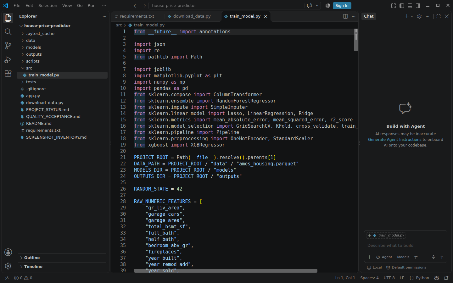
Real Visual Studio Code window showing src/train_model.py from the House Price Predictor project — Real project file opened in Visual Studio Code after the verified build. The complete copyable source is shown above.

Check before continuing: src/train_model.py exists, is saved, and contains the complete code below.

See what the preprocessing pipeline is doing

Imputation means filling a missing value using a rule learned from available data. Numeric fields use the median. Categorical fields use the most frequent value.

One-hot encoding converts a category such as a neighborhood into numeric indicator columns.Standard scaling puts numeric values on comparable scales for the linear models.

The important safety detail is that these steps live inside a scikit-learn Pipeline andColumnTransformer. During cross-validation, preprocessing is fitted inside each training fold. That prevents information from the validation fold leaking into the model.

The project also creates three understandable features: house age at sale, years since remodel, and total bathrooms where a half bath counts as 0.5.

Check before continuing: You understand that imputation, scaling and encoding are learned using training folds rather than the final test set.

Keep the final test set untouched

The program first separates 20% of the rows into a holdout test set. Think of this as a sealed exam paper. We do not use it to choose the winner.

The remaining 80% is used for model comparison. Five-fold cross-validation repeatedly trains on four parts and validates on the fifth part, rotating the validation part five times. This gives a more stable comparison than one lucky split.

Our primary comparison metric is RMSE — Root Mean Squared Error. Lower is better. RMSE gives larger mistakes extra weight because errors are squared before being averaged.

Check before continuing: You know why we do not repeatedly choose the winner by looking at the final test score.

Train and compare five regression models

Run the complete training program from the project root:

Train the projectpowershellRunnable

python src/train_model.py

The verified build produced this training-only cross-validation comparison:

Real 5-fold CV resulttextOutput

Model              CV RMSE    CV MAE    CV R²
XGBoost             $26,575    $16,867   0.874
Random Forest       $27,585    $17,438   0.867
Ridge               $31,214    $19,154   0.825
Linear Regression   $31,251    $18,887   0.824
Lasso               $31,562    $19,432   0.820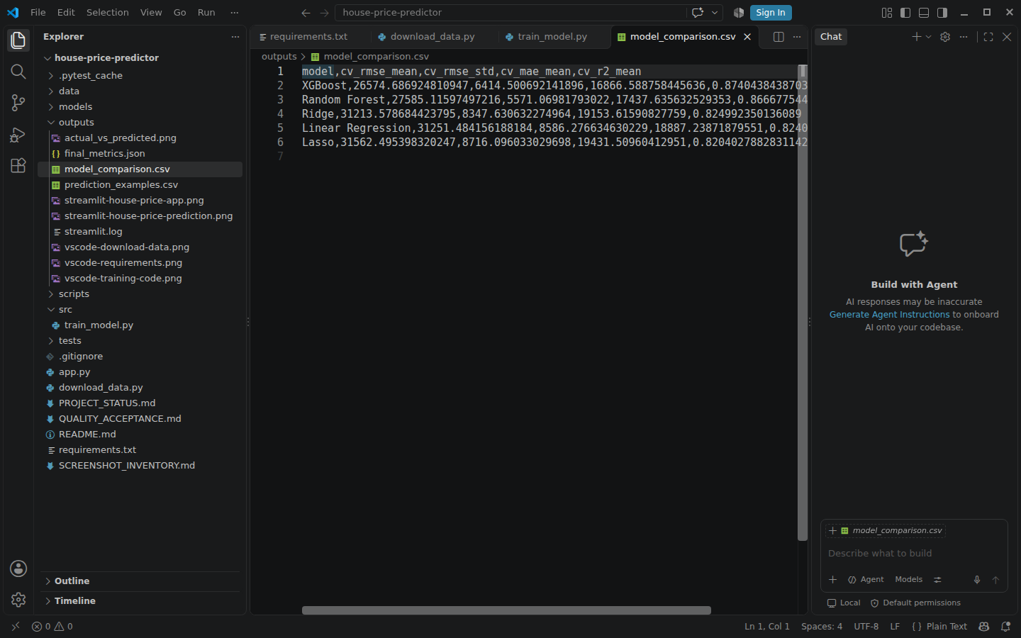

Real Visual Studio Code window showing the generated model_comparison.csv from the verified training run — The file was produced by the real five-model cross-validation run. It is evidence from the executable project, not an illustrative table.

XGBoost had the lowest mean CV RMSE, so it became the model to tune. Notice that we did notinspect the final holdout test scores to choose the winner.

Check before continuing: The command completes and outputs a five-row comparison table.

Tune XGBoost using training data only

A hyperparameter is a setting chosen before model fitting. The project tries a small, reproducible grid of XGBoost settings using cross-validation on the training data.

The verified run selected:

Real tuning resulttextOutput

learning_rate = 0.06
max_depth = 3
n_estimators = 450
best cross-validation RMSE = $26,542

This is intentionally a small educational search, not an expensive competition-scale tuning exercise.

Check before continuing: Your run reports XGBoost as the selected model and finishes the tuning stage before holdout evaluation.

Evaluate the final model once on the holdout set

Real verified holdout outputtextOutput

Final holdout evaluation (used once after model selection/tuning):
MAE:  $15,670
RMSE: $23,792
R²:   0.929

Saved model: .../models/house_price_pipeline.joblib
Reload check prediction: $153,563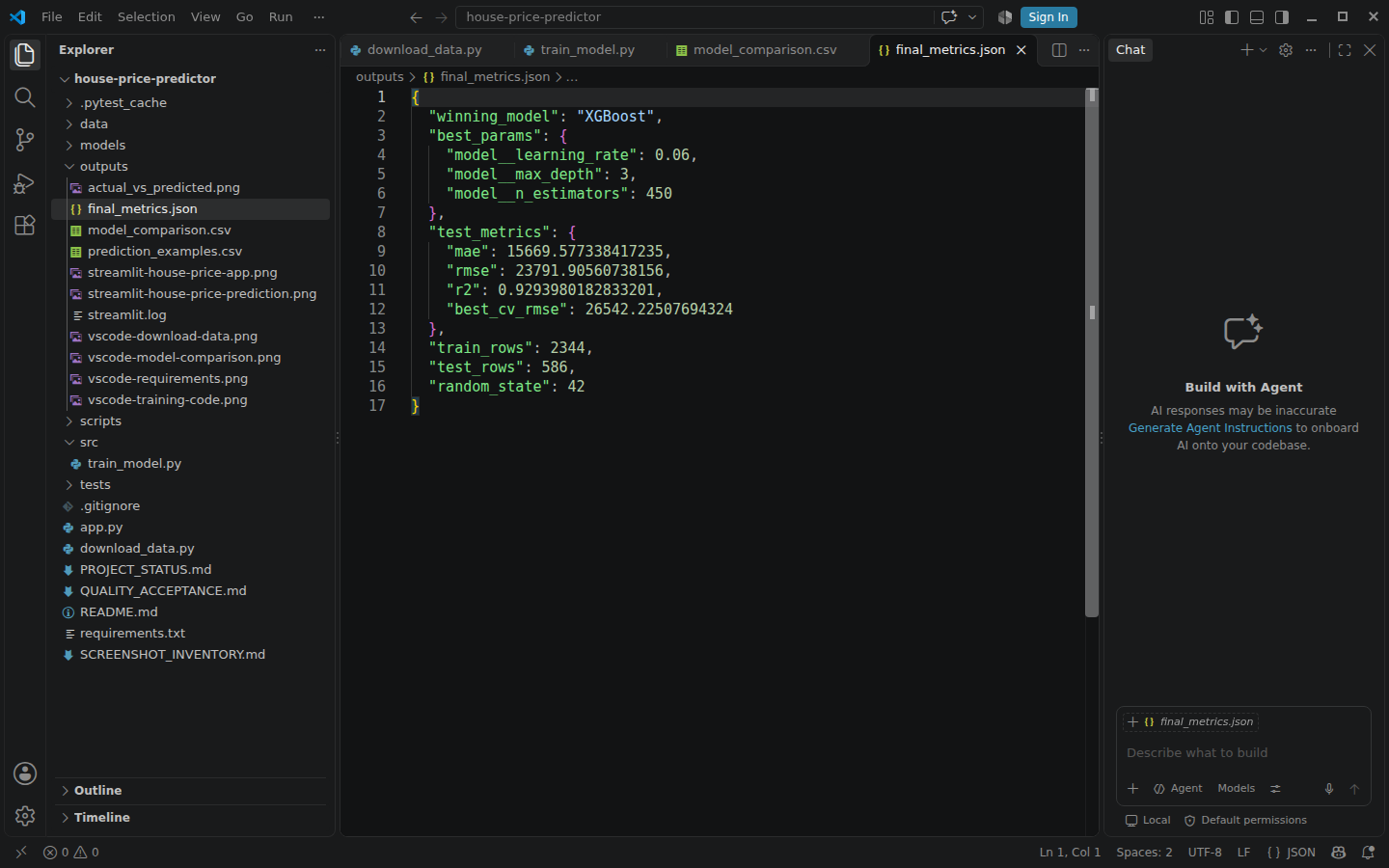

Real Visual Studio Code window showing final_metrics.json from the verified House Price Predictor holdout evaluation — The generated metrics file records the selected model, tuned settings, final holdout metrics, row counts and random seed from the verified run.

MAE $15,670 means the absolute prediction error is about $15,670 on average in this test set.RMSE $23,792 penalizes larger errors more strongly. R² 0.929 means the model explains about 92.9% of the variation in sale prices in this held-out sample.

These metrics describe this historical dataset and split. They do not mean the application is a certified property appraisal system.

Check before continuing: Your final output reports MAE, RMSE and R² and saves models/house_price_pipeline.joblib.

Read the Actual vs Predicted chart

The training program saves outputs/actual_vs_predicted.png. Each dot is one held-out house. The horizontal position is the real sale price. The vertical position is the model's prediction.

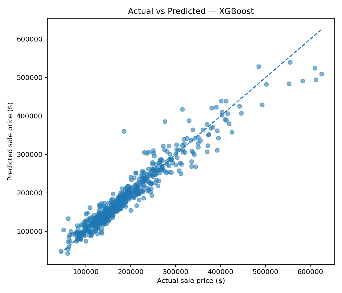
Actual versus predicted sale-price scatter plot from the verified XGBoost holdout evaluation

The dashed diagonal is perfect prediction. Most points follow that diagonal closely, while some expensive homes show larger errors. That is one reason we report multiple metrics instead of claiming the model is perfect.

Check before continuing: You can explain why points closer to the dashed diagonal represent better predictions.

Create the Streamlit browser application

Streamlit turns Python code into a browser interface. Create app.py in the project root and paste the complete verified application:

app.py — complete Streamlit applicationpythonRunnable

from __future__ import annotations

import json
from pathlib import Path

import joblib
import pandas as pd
import streamlit as st

PROJECT_ROOT = Path(__file__).resolve().parent
MODEL_PATH = PROJECT_ROOT / "models" / "house_price_pipeline.joblib"
METADATA_PATH = PROJECT_ROOT / "models" / "app_metadata.json"


@st.cache_resource
def load_artifacts():
    if not MODEL_PATH.exists() or not METADATA_PATH.exists():
        raise FileNotFoundError(
            "The trained model is missing. Run python download_data.py and then python src/train_model.py."
        )

    model = joblib.load(MODEL_PATH)
    metadata = json.loads(METADATA_PATH.read_text(encoding="utf-8"))
    return model, metadata


def build_model_row(raw_values: dict) -> pd.DataFrame:
    row = pd.DataFrame([raw_values])

    row["house_age_at_sale"] = row["year_sold"] - row["year_built"]
    row["years_since_remodel"] = row["year_sold"] - row["year_remod_add"]
    row["total_bathrooms"] = row["full_bath"] + (0.5 * row["half_bath"])

    model_columns = [
        "gr_liv_area",
        "garage_cars",
        "garage_area",
        "total_bsmt_sf",
        "bedroom_abv_gr",
        "fireplaces",
        "lot_area",
        "house_age_at_sale",
        "years_since_remodel",
        "total_bathrooms",
        "neighborhood",
        "house_style",
        "kitchen_qual",
        "overall_qual",
    ]
    return row[model_columns]


st.set_page_config(
    page_title="House Price Predictor",
    page_icon="🏠",
    layout="centered",
)

st.title("🏠 What Is This House Really Worth?")
st.caption("A beginner-friendly Ames Housing machine-learning project")

try:
    model, metadata = load_artifacts()
except FileNotFoundError as error:
    st.error(str(error))
    st.stop()

st.info(
    "Educational demo only. The model uses historical home sales from Ames, Iowa, "
    "and is not a professional appraisal or a current market valuation."
)

with st.expander("About the trained model", expanded=False):
    metrics = metadata["final_metrics"]
    st.write("Selected model:", metadata["winning_model"])
    st.write("Holdout MAE: $" + f"{metrics['mae']:,.0f}")
    st.write("Holdout RMSE: $" + f"{metrics['rmse']:,.0f}")
    st.write(f"Holdout R²: {metrics['r2']:.3f}")

defaults = metadata["numeric_defaults"]
categories = metadata["categorical_options"]

st.subheader("Enter the property details")

col1, col2 = st.columns(2)

with col1:
    gr_liv_area = st.number_input(
        "Above-ground living area (sq ft)",
        min_value=300,
        max_value=6000,
        value=int(defaults["gr_liv_area"]["median"]),
        step=50,
    )
    lot_area = st.number_input(
        "Lot area (sq ft)",
        min_value=1000,
        max_value=100000,
        value=int(defaults["lot_area"]["median"]),
        step=250,
    )
    total_bsmt_sf = st.number_input(
        "Basement area (sq ft)",
        min_value=0,
        max_value=5000,
        value=int(defaults["total_bsmt_sf"]["median"]),
        step=50,
    )
    garage_area = st.number_input(
        "Garage area (sq ft)",
        min_value=0,
        max_value=2000,
        value=int(defaults["garage_area"]["median"]),
        step=25,
    )
    garage_cars = st.number_input(
        "Garage capacity (cars)",
        min_value=0,
        max_value=5,
        value=int(round(defaults["garage_cars"]["median"])),
        step=1,
    )
    bedrooms = st.number_input(
        "Bedrooms above ground",
        min_value=0,
        max_value=8,
        value=int(round(defaults["bedroom_abv_gr"]["median"])),
        step=1,
    )

with col2:
    full_bath = st.number_input(
        "Full bathrooms",
        min_value=0,
        max_value=5,
        value=int(round(defaults["full_bath"]["median"])),
        step=1,
    )
    half_bath = st.number_input(
        "Half bathrooms",
        min_value=0,
        max_value=4,
        value=int(round(defaults["half_bath"]["median"])),
        step=1,
    )
    fireplaces = st.number_input(
        "Fireplaces",
        min_value=0,
        max_value=5,
        value=int(round(defaults["fireplaces"]["median"])),
        step=1,
    )
    year_built = st.number_input(
        "Year built",
        min_value=1870,
        max_value=2010,
        value=int(round(defaults["year_built"]["median"])),
        step=1,
    )
    year_remodeled = st.number_input(
        "Year last remodeled",
        min_value=1870,
        max_value=2010,
        value=int(round(defaults["year_remod_add"]["median"])),
        step=1,
    )
    year_sold = st.number_input(
        "Year sold",
        min_value=2006,
        max_value=2010,
        value=int(round(defaults["year_sold"]["median"])),
        step=1,
    )

neighborhood = st.selectbox("Neighborhood", categories["neighborhood"])
house_style = st.selectbox("House style", categories["house_style"])
kitchen_qual = st.selectbox("Kitchen quality", categories["kitchen_qual"])
overall_qual = st.selectbox("Overall quality", categories["overall_qual"])

raw_values = {
    "gr_liv_area": float(gr_liv_area),
    "garage_cars": float(garage_cars),
    "garage_area": float(garage_area),
    "total_bsmt_sf": float(total_bsmt_sf),
    "full_bath": float(full_bath),
    "half_bath": float(half_bath),
    "bedroom_abv_gr": float(bedrooms),
    "fireplaces": float(fireplaces),
    "year_built": float(year_built),
    "year_remod_add": float(year_remodeled),
    "year_sold": float(year_sold),
    "lot_area": float(lot_area),
    "neighborhood": neighborhood,
    "house_style": house_style,
    "kitchen_qual": kitchen_qual,
    "overall_qual": overall_qual,
}

if st.button("Estimate sale price", type="primary", use_container_width=True):
    if year_remodeled < year_built:
        st.warning("The remodel year cannot be earlier than the build year.")
    elif year_sold < year_built:
        st.warning("The sale year cannot be earlier than the build year.")
    else:
        model_row = build_model_row(raw_values)
        prediction = float(model.predict(model_row)[0])
        st.metric("Estimated historical sale price", "$" + f"{prediction:,.0f}")
        st.caption(
            "This estimate is based on patterns in the historical Ames Housing dataset. "
            "It does not adjust the old sale prices to today's dollars."
        )

How the application code works

1. load_artifacts() loads the saved pipeline and metadata. If training has not created them, the app stops with a useful message rather than producing a fake prediction.

2. Streamlit input widgets collect the same raw property information used by the training project: area, garage, bathrooms, years, neighborhood and quality fields.

3. build_model_row() recreates only the deterministic engineered features—house age, years since remodel and total bathrooms—and orders the columns exactly as the saved pipeline expects.

4. model.predict() sends that one-row DataFrame through the saved preprocessing steps and then through XGBoost. The app itself does not refit imputation, encoding, scaling or the model.

5. st.metric() displays the prediction. The warning below it reminds the learner that the Ames dataset contains historical prices and is not a current professional appraisal.

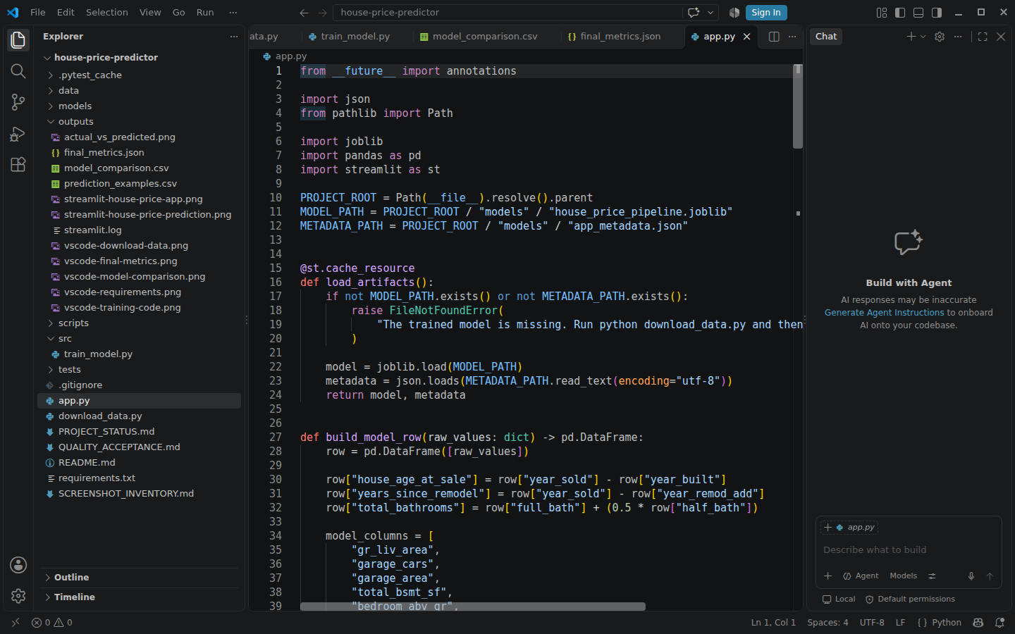
Real Visual Studio Code window showing app.py for the verified Streamlit House Price Predictor — Real application source opened in Visual Studio Code. The complete copyable code is directly above this screenshot.

The app loads the saved preprocessing-and-model pipeline. This is important: it does not try to recreate preprocessing rules separately at prediction time.

Check before continuing: app.py exists at the project root and contains the complete code below.

Run the application and make a prediction

From the project root, run:

Start the browser applicationpowershellRunnable

streamlit run app.py

Streamlit prints a local address, normally http://localhost:8501. Ctrl+click that address in the terminal, or copy it into your browser.

Leave the default values first.
Scroll down to Estimate sale price.
Click the button.
A price estimate should appear below it.

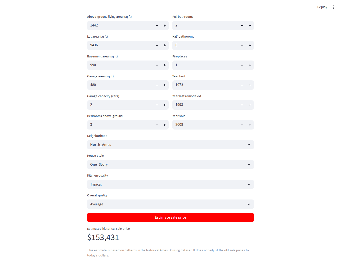
Real House Price Predictor Streamlit result showing an estimated historical sale price

In our verified screenshot, the default form produced an estimated historical sale price of $153,431. The earlier command-line reload check used a different test row and produced $153,563; those are two different predictions, not a contradiction.

Check before continuing: A browser page opens and Estimate sale price returns a dollar estimate without an exception.

Add an automated app smoke test

A smoke test is a quick check that the application can start without crashing. Createtests/test_app.py and paste:

tests/test_app.pypythonRunnable

from pathlib import Path

from streamlit.testing.v1 import AppTest

PROJECT_ROOT = Path(__file__).resolve().parents[1]


def test_streamlit_app_loads_without_exception():
    app = AppTest.from_file(str(PROJECT_ROOT / "app.py"), default_timeout=30)
    app.run()
    assert not app.exception
    assert any("What Is This House Really Worth?" in title.value for title in app.title)

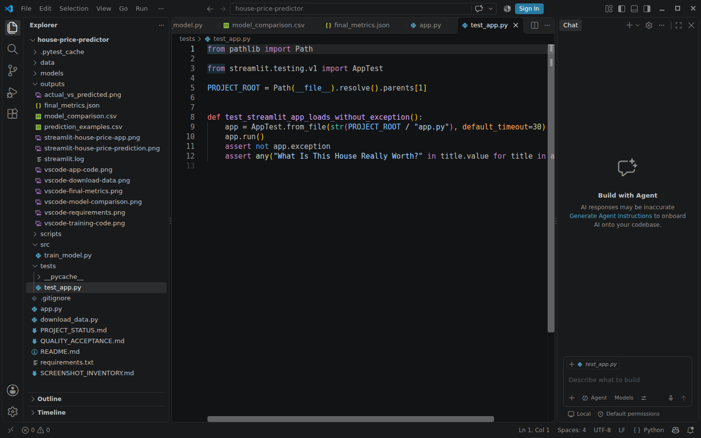
Real Visual Studio Code window showing tests/test_app.py for the House Price Predictor — The smoke test shown here is the same test executed by the verified project workflow.

Then run:

Run the smoke testpowershellRunnable

pytest -q

Verified test resulttextOutput

.                                                                        [100%]
1 passed

Check before continuing: pytest -q reports one passing test.

Understand the complete project folder

house-price-predictor/
├── data/
│   └── ames_housing.parquet
├── models/
│   ├── house_price_pipeline.joblib
│   └── app_metadata.json
├── outputs/
│   ├── actual_vs_predicted.png
│   ├── final_metrics.json
│   ├── model_comparison.csv
│   └── prediction_examples.csv
├── src/
│   └── train_model.py
├── tests/
│   └── test_app.py
├── app.py
├── download_data.py
├── requirements.txt
├── README.md
└── .gitignore

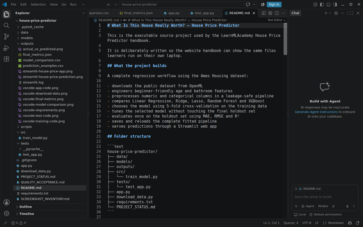
Real Visual Studio Code workspace for the completed House Price Predictor project — Final verified project workspace in Visual Studio Code. Generated data, model and output folders appear only after their earlier commands have run successfully.

Files in data, models and outputs are generated from the reproducible source project. The Python source and dependency file are the important things to preserve in version control.

Check before continuing: Your important files match this structure and generated folders contain the model and outputs.

Put the finished project on GitHub

Do this only after the project works locally. Install Git for Windows from the official Git for Windows page.

First create .gitignore. This prevents the virtual environment, downloaded dataset, trained model and generated outputs from being added to Git accidentally.

.gitignore — copy this exactlytextConfiguration

.venv/
__pycache__/
.pytest_cache/
data/*.parquet
data/*.csv
models/*.joblib
models/*.json
outputs/*.csv
outputs/*.json
outputs/*.png

Next create README.md. This is the page a recruiter or another learner sees first when opening your GitHub repository. Start with the complete portfolio-ready version below; after you finish the exercises, add what you changed and what happened.

README.md — project explanationmarkdownConfiguration

# House Price Predictor

A complete regression project using the Ames Housing dataset.

## What it does
The project compares five regression model families, tunes the best one using training-only cross-validation, evaluates it once on an untouched holdout set, saves the complete preprocessing + model pipeline, and serves predictions through Streamlit.

## Tools
Python, Pandas, NumPy, scikit-learn, XGBoost, Joblib, Matplotlib, Streamlit, Pytest

## Run
```powershell
python download_data.py
python src/train_model.py
pytest -q
streamlit run app.py
```

## Verified reference result
- Winner: XGBoost
- Holdout MAE: $15,670
- Holdout RMSE: $23,792
- Holdout R²: 0.929

## Important limitation
This is an educational model trained on historical Ames, Iowa sales. It is not a current professional property appraisal.

Now create an empty repository on GitHub and use the commands below. Replace the example remote URL with the URL GitHub shows for your repository.

Git/GitHub commandspowershellRunnable

git init
git add .
git status
git commit -m "Build house price predictor"
git branch -M main
git remote add origin https://github.com/YOUR-USERNAME/house-price-predictor.git
git push -u origin main

Before git commit, always read the output of git status. Do not commit passwords, API keys or your .venv folder.

Check before continuing: Your GitHub repository shows the source files and does not contain .venv or generated model/data files.

Common problems and fixes

python is not recognized: reopen PowerShell after Python installation. If needed, repair/reinstall Python and enable command-line/PATH integration.

Activate.ps1 cannot be loaded: use Set-ExecutionPolicy -Scope Process -ExecutionPolicy Bypass in that terminal, then activate again.

ModuleNotFoundError: confirm (.venv) appears in your prompt, then rerun pip install -r requirements.txt.

ames_housing.parquet does not exist: run python download_data.py from the project root before training.

python cannot open src/train_model.py: run dir. You are probably in the wrong folder. Navigate back to the project root.

Streamlit says the model is missing: training did not finish successfully. Rerun python src/train_model.py and verify the saved-model line appears.

App opens but prediction fails after you changed features: the app inputs must match the columns the saved pipeline expects. Retrain and update the app together.

Now change the project yourself

Copying the finished code proves you can reproduce the build. The exercises below prove you understand it. Make one change at a time, rerun training, and compare the result with the verified baseline above.

Exercise 1 — Remove one useful feature

Temporarily remove garage_cars from the raw/model feature lists, retrain, and compare CV RMSE. The goal is not to force a worse score; it is to see that features are choices whose value can be tested.

Exercise 2 — Change the XGBoost search

Add max_depth = 4 to the tuning grid. Rerun and inspect the best parameters and CV RMSE. A larger search is not automatically better; you are testing whether extra complexity helps validation performance.

Exercise 3 — Trace one prediction end to end

Choose one set of values in Streamlit. Identify which raw fields enter build_model_row(), which three engineered values are created, and where the saved pipeline receives the final row.

Exercise 4 — Break it on purpose

Rename models/house_price_pipeline.joblib temporarily and run the app. Read the error, restore the filename, and rerun. This teaches you how the application depends on the trained artifact.

How to explain this project in an interview

Why did you use a scikit-learn Pipeline?

To keep imputation, encoding/scaling and the estimator together so every validation fold learns preprocessing only from its training portion, and so inference uses the exact fitted transformations.

Why did you keep a holdout set?

Cross-validation was used to compare and tune models. The holdout stayed untouched so the final reported result came from data that did not influence those decisions.

Why was RMSE the primary selection metric?

House-price errors are measured in dollars, and RMSE gives larger mistakes more weight. We also report MAE and R² so one metric does not tell the whole story.

Why did XGBoost win?

It produced the lowest mean 5-fold CV RMSE among the five candidate model families in this verified run. It was selected by validation evidence, not by brand or popularity.

How did you avoid training-serving mismatch?

The whole fitted preprocessing + model pipeline was saved with Joblib. The Streamlit app loads that artifact instead of rebuilding preprocessing separately.

What is the biggest limitation?

The data describes historical sales in Ames, Iowa. The model is not adjusted to today’s dollars, other cities or changing market conditions, so it is an educational estimator rather than a real appraisal product.

What would change for a real production system?

A notebook-quality score is not enough for a production appraisal product. Before real use you would need fresher geographically relevant sales data, stronger data-quality checks, inflation/market-time treatment, outlier analysis, fairness and subgroup checks, monitored prediction/error drift, versioned model releases, automated retraining rules, authentication and logging, and a clear human-review process for high-value decisions.

Streamlit is perfect for learning and demos. A production service might instead expose the model through an API, validate requests with a schema, store model/version metadata with each prediction and place a separate web or mobile interface in front of that API.

Implementation mastery check

Do not call the project finished just because the app opens. You should be able to answer these without looking at the code.

What exactly is the prediction target?

Which inputs are numeric and which are categorical?

Which three features do we engineer and how?

Why is preprocessing kept inside the pipeline?

What would data leakage look like in this project?

Why do we compare models with cross-validation?

Why is the holdout used only after selection/tuning?

What do MAE, RMSE and R² each tell you?

Why was XGBoost selected in this run?

What exactly is stored in house_price_pipeline.joblib?

How does app.py transform one user form submission into a model input?

Why can the same saved pipeline accept a new neighborhood category safely?

How would you debug a missing model-file error?

What would you change before using this outside historical Ames data?

Complete-project checkpoint

Official Ames Housing data downloaded

Five regression models compared with cross-validation

Final holdout kept untouched during selection

XGBoost tuned on training data only

MAE, RMSE and R² reported

Complete preprocessing + model pipeline saved

Saved pipeline reloaded successfully

Streamlit app runs in the browser

Automated app test passes

Real result screenshots captured

All important code is visible in this handbook

Project is ready to place on GitHub

What you have learned

You did much more than call model.fit(). You created a reproducible project, obtained real data, separated training and final evaluation correctly, handled numeric and categorical preprocessing without leakage, compared several regression families, tuned a winner, interpreted real metrics, saved the whole pipeline and put the model behind a browser interface.

That end-to-end workflow is the main purpose of this handbook. You should now be able to open your own folder and point to the exact file responsible for data acquisition, training, evaluation, persistence, testing and inference.